Introduction to Vehicle Dynamics Using MATLAB

• How to drive these vehicles automatically?
• How to reduce traveling time?

The second most important milestone was achieved with the invention of steam engines. Vehicles now can be driven automatically. Followed by steam engines invention of the Internal Combustion engine happened. These engines are used to convert potential energy in the form of water/heat or petrol into mechanical energy which is then transferred to wheels to move vehicles faster. In recent times there is an increased demand for vehicle safety, environmental concerns and intelligent control. Software were also introduced into vehicles to control mechanical aspects more accurately, and Electrical engines are invented to address environmental concerns. Even though we have come across a long way of invention but still there is plenty of room available for improvement as new challenges are coming across. Therefore, it is essential to understand what the vehicle is constituted of and how it will behave provided different scenarios in the outer environment.

Introduction to Vehicle Dynamics

• Studying the behavior of vehicles or Integrated subsystems of vehicles under given circumstances is referred to as Vehicle Dynamics.

Analysis of Vehicle dynamic response requires implementing vehicles' different subsystems in the form of mathematical representation to understand different forces acting on vehicles. As these mathematical representations are quite complex, we need a tool where we can implement these equations easily and simulate them in a faster way. There are different simulators available that can help us to achieve the same.

1. ADAMS: The multibody dynamics simulation tool, can help us study systems with multiple moving parts such as robots.
2. Carmaker & Carsim: These tools can be used to perform analysis of vehicles using different simulations followed by tuning the parameters using the API provided.
3. MATLAB: Since we will be implementing subsystems of vehicles ourselves, we need a tool that has the capability to represent and solve the equations very easily with its ability to handle trigonometry, linear algebra and kinematics. So, we will take the help of MATLAB to assist us in this analysis.

Along with the above benefits, MATLAB also has advanced toolboxes to understand this topic in further details.

Keywords: Vehicle Dynamics, state space, Bicycle Model, Ackerman’s criteria, OEM, ADAS, Understeer gradient.

Target Audience

Knowledge of vehicle dynamics is helpful to peruse a carrier in the tire, suspension, braking and transmission design. In the Automotive industry to develop ADAS applications. For example, Lane Keep Assist, Lane centering, Automatic cruise control and many more. So Engineering students from Computer science, electronics/electrical and mechanical branch & all those who are enthusiastic about the automotive industry can take this course.

Prerequisites

Along with basic scripting knowledge of MATLAB and Simulink, introductory knowledge of linear algebra and planar geometry will be required to understand the topics throughout. Understanding and state space representation of equations will be described while discussing the demo for each subsystem.

We will start our first lesson by identifying the most important aspects which contribute to vehicles' behavior when it’s on the move. The below section will provide more regarding them. Before explaining the subsystems of vehicles, let us understand a few terminologies involved in vehicles' motion.

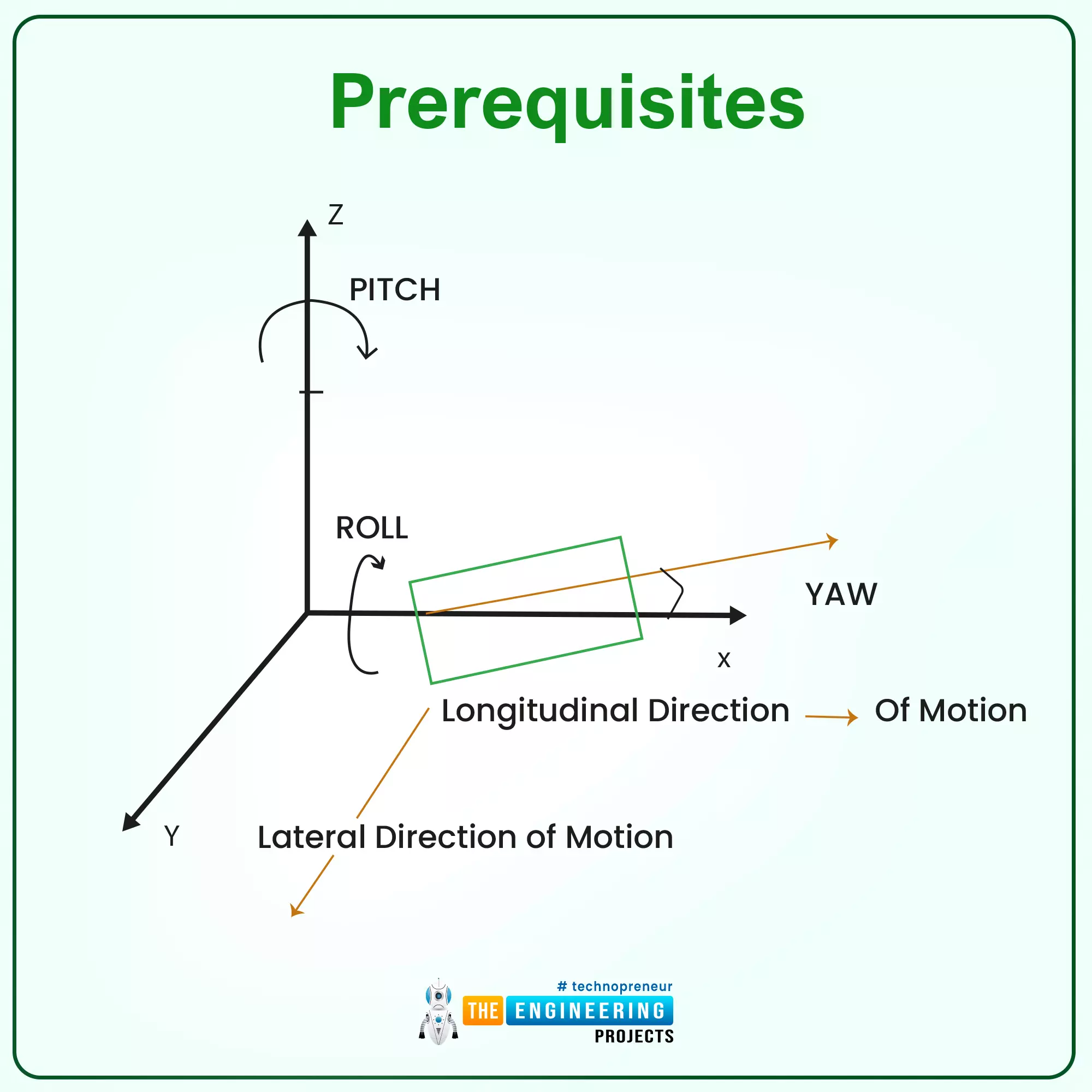
• Vehicle motion along X-Axis is called longitudinal motion, and angle across X-Axis is called roll.
• And vehicle motion in the direction towards Y-axis is called lateral motion and angle is called Yaw

Since vehicles can travel either to the left or to the right study of motion along the Z-axis is not required to consider.

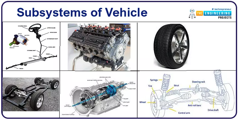
Subsystems of Vehicle

To simplify the mathematical models involved and describe concepts in their simplistic form we will focus on subsystems that are applicable to both commercial and passenger vehicles. From a broader perspective, the performance of a vehicle can be affected due to 7 different subsystems,

Figure 1: Vehicle Dynamics Subsystems

• Road – Performance of vehicles on a different set of roads is not shown in the diagram as roads are not part of the vehicle body itself. But as they affect how the vehicles perform. We shall prepare the mathematics model and its elements involved in our study.

1. Lateral Dynamics

To understand the need for lateral dynamics let us take an example, that car is traveling on a circular road.

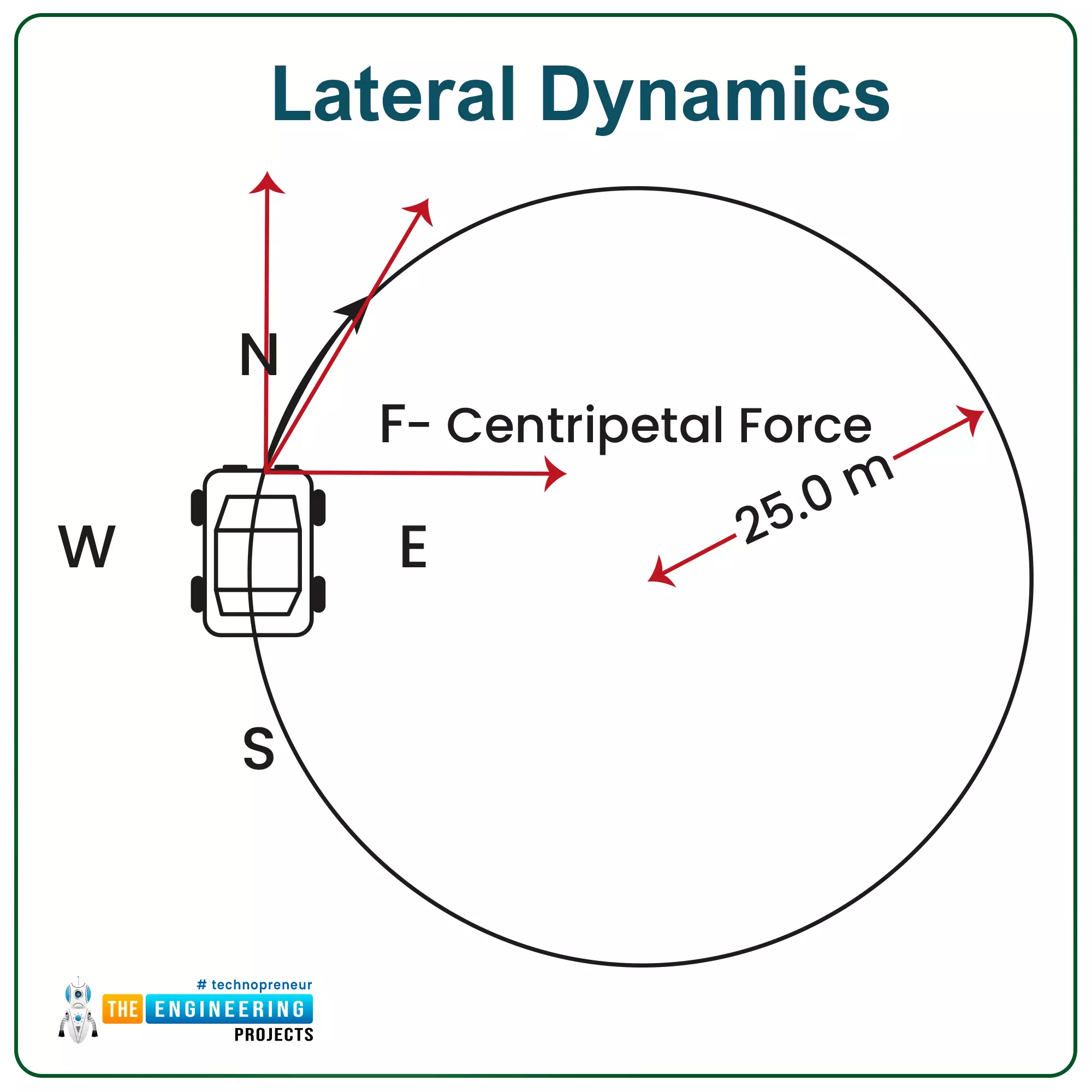
The force vector shown on the line of the circle can be separated into two components, one component normal to X-Axis and another along the X-axis. The amount of force along the X-axis will be responsible to pull the vehicle towards the center of the circle. Because of which driver will feel that vehicle is going outside of the road. This phenomenon was first observed in the 17^th century and a study for Vehicles traveling on the circular road with constant velocity and constant steering was started. To prevent the vehicle from going out of the road, an equal amount of force is needed which will push the vehicle outwards, called centrifugal force.

This behavior in which it appears like the vehicle is going to leave the road due to less steering is called understeering. In a similar way, the oversteering phenomenon can be observed. The output of the lateral or steering subsystem decides how the vehicle will behave in the lateral direction, while in motion. The lateral dynamics of vehicles can be studied by building a kinematic model, by building meaning implementing geometric equations in MATLAB. To understand these kinematic equations we will be referring to planar geometry, where we consider vehicle motion in the (X, Y) axis.

Even if take passenger vehicle, which has 4 wheels, components involved in modeling 4 wheels are complex as the four different delta angles of wheels and their dimensions will have an impact.

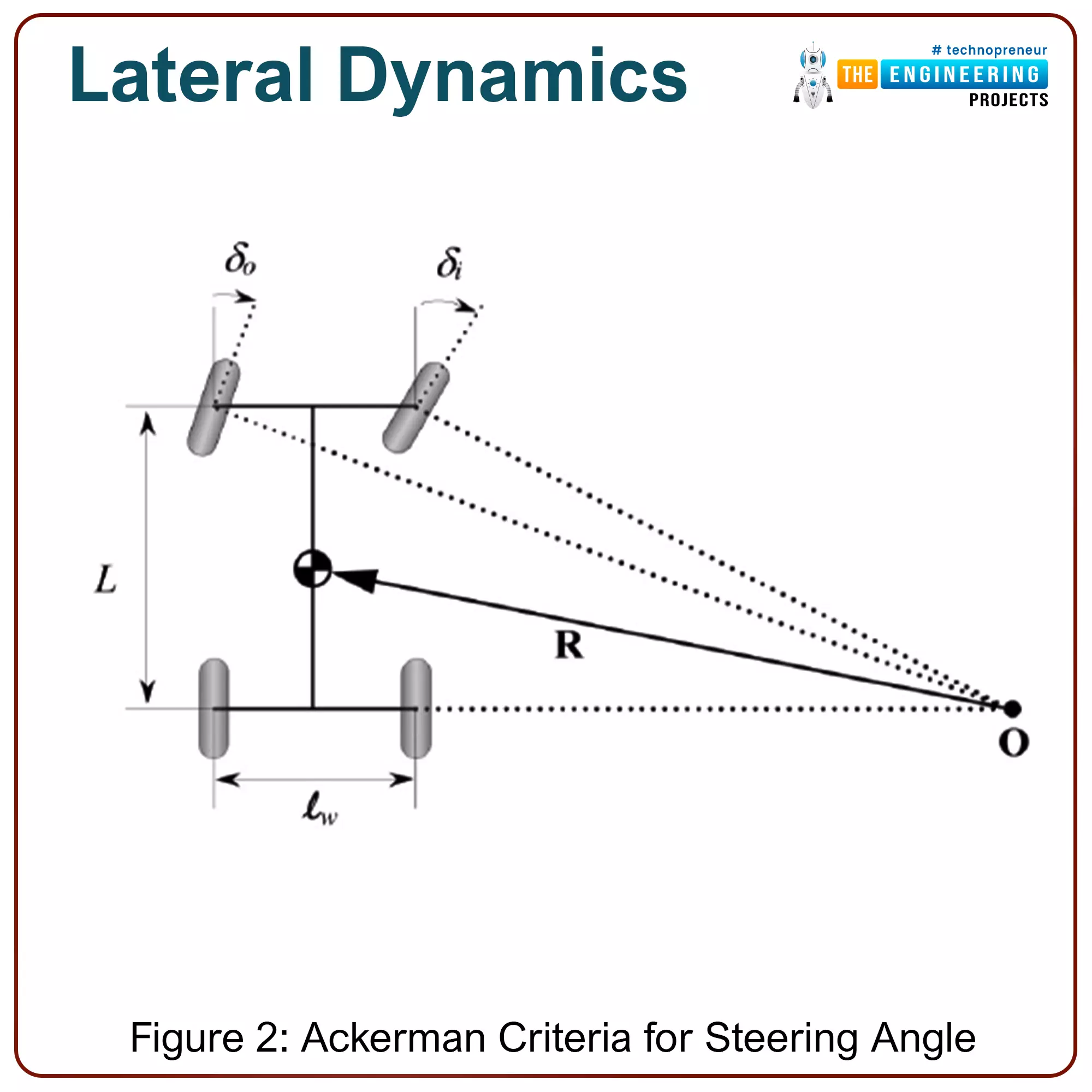
Figure 2: Ackerman Criteria for Steering Angle

So, to make the initial study simpler we will make a few assumptions.

1. Let us assume that the left and right half parts of the vehicle behave in a similar manner.
2. The second assumption is that only front wheels can move independently, meaning steering can control the movement of front wheels (Popularly known as front-wheel-drive system). Wheels on the rear side will follow the course.

With this assumption, we can combine the left and right parts and consider that the vehicle has only two wheels one on the front side and another at the back.

This model is called a bicycle model as it looks like a bicycle. And as we can observe the complexity involved in the model is also reduced. The bicycle model has a “Two” degree of freedom (Y, ?). Where theta being angle with respect to Y-axis or Yaw of vehicle.

The assumption involved mainly considering both left-hand and right-hand side wheel takes same steering angle, hence represented with a single wheel. However, the steering angle provided to left- and right-hand side wheels are slightly different due to the radius they must cover.

As seen in the image, R corresponds to the radius to be covered resulting in the wheel angle delta provided using steering. Ackerman’s equations will help in analyzing scripted bicycle models on different curvatures. And length “a” is the length of the shaft from the center of gravity to the front wheel. “b” is the length of the driving shaft from the center of gravity to the rear wheel.

2. Longitudinal Dynamics

Just now we had introduced a subsystem of vehicles that affects the behavior of vehicles during lateral motion. Our second subsystem contributes in the longitudinal direction. As shown above, the longitudinal subsystem is made up of 3 parts.

1. The engine generates the necessary power to drive the vehicle.
2. Torque converter converts this power to drive mechanical components such as drive shaft, ensuring the comfort of persons sitting inside the vehicle. For example, a torque converter acts to reduce the torque transferred from the engine to the transmission unit when the driver is pressing a break.
3. A transmission unit: Gears, clutch and torque distribution to wheels.

The torque output performance of the engine can be studied using parameterized models and maps of thrust to exhaust for every paddle position on the accelerator proposed as outputs.

2.1. Engine

The engine serves as a vehicle's power source. Understanding of engine characteristics is tightly coupled with the transmission. In layman’s term engines are characterized by power it provides generated torque at different speed or throttle/accelerator position.

Torque= Generated power X Speed of vehicle

Also, to determine acceleration performance it is important to analyze the power/weight ratio of vehicles. Which can be determined by using Newton’s second law of motion. We shall study braking performance implementing the same law of motion.

2.2. Transmission

Since vehicles may travel on a surface which is having a certain amount of slope. It is very important to ensure that the maximum amount of torque produced by the vehicle is transferred to the wheels. Gears were invented to satisfy this need. These parts having teeth are used to convert the rotational motion of the shaft to a translational one so that it can be provided to wheels. Gears are also used to change the direction of power distribution, which helps in driving a vehicle in the reverse direction.

Above are a couple of examples to understand the importance of transmission to move vehicles in the longitudinal direction. Now let us consider a case, where while traveling in turn vehicle’s outer wheel shall move faster than the inner wheel. It is because the outer wheel needs to travel more distance than the inner wheel as the radius of the curve is different.

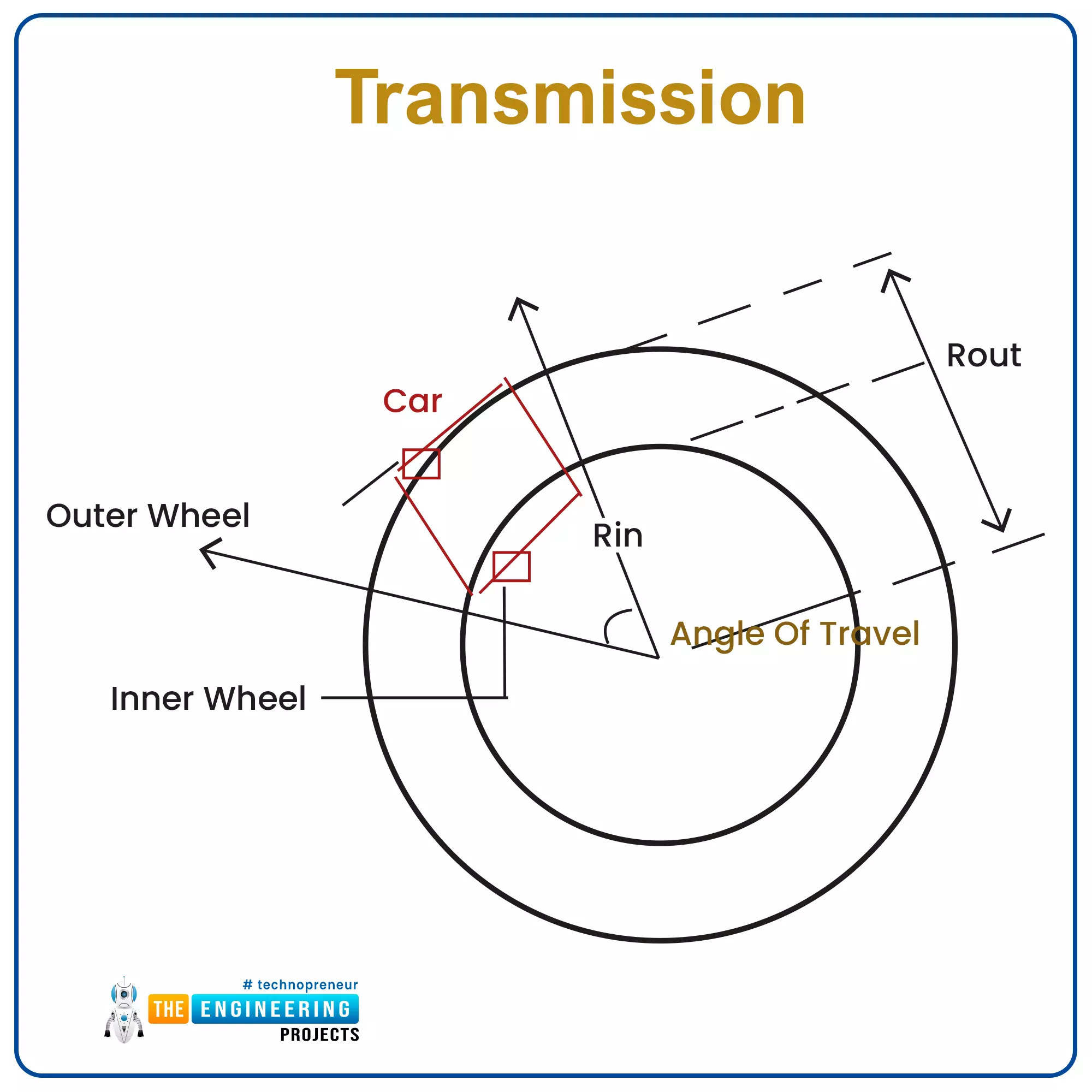
• Distance travelled by inner wheel = 2* Angle of travel * Rin.
• Distance travelled by inner wheel = 2* Angle of travel * Rout.

To satisfy this constraint differential torque distribution is used by the Transmission unit. We will study how gears help in providing different torque to wheels on each side to meet this demand. This differential torque distribution can be demonstrated using the Simulink Simscape product from the MATLAB family of work products. The image is shown here, enlists a few block sets involved in modeling.

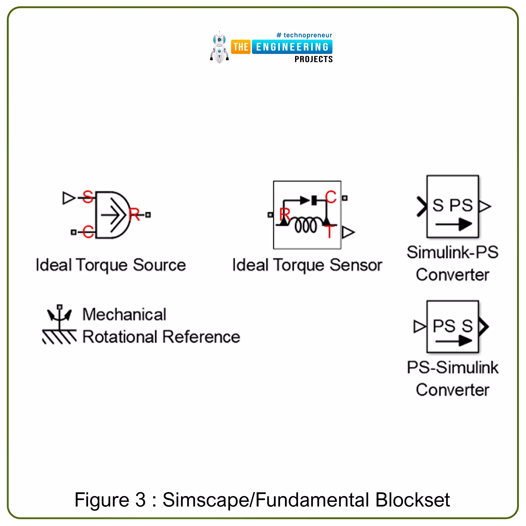
Figure 3: Simscape/Fundamental Blockset

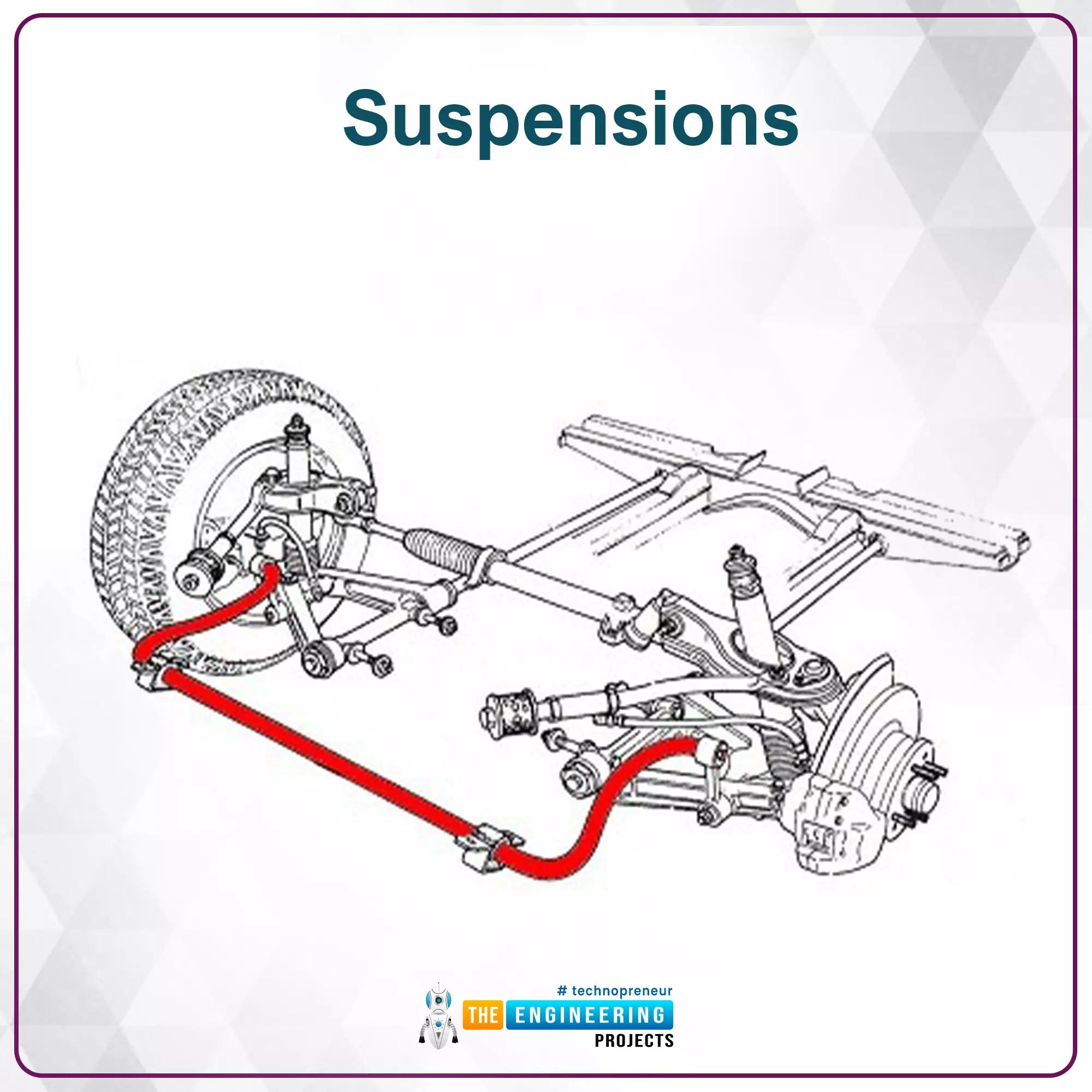
3. Suspensions

As the basic requirements are satisfied with lateral and longitudinal dynamics. The third subsystem focuses on the comfort provided to passengers while moving. Vehicle suspension functionality is to support the body of the vehicle over its chassis. In mechanical terms suspension of a vehicle helps in defining vehicle Ride, Roll and handling. The vehicle is categorized as good or bad comfort based on two aspects. How easy the vehicle is to steer; does it provide a comfortable acceleration and braking experience to the driver.

• Ride: For better ride comfort vehicle suspension shall isolate the body of the vehicle from the chassis so that acceleration and jerk experience reduce to its minimum.

For example, consider the vehicle is traveling at a speed of 100kph speed. And the driver applies the brake. Now due to inertia, if the vehicle stops very aggressively then it might give an uncomfortable experience to passengers sitting inside, meanwhile, it is also important to stop the vehicle at a minimum distance as possible.

• Roll: The roll of the vehicle can define how effectively a vehicle can hold the ground at maximum lateral acceleration. It's expected that the vehicle tire on the outside shall always be grounded while corning.

To increase rolling capacity one of the mechanical methods used is “Anti Roll Bar”.

Steering Step Response or vehicle Cornering test is used where the vehicle is driven at different high speeds and the steering wheel is rotated suddenly in one direction to check if the vehicle left the ground.

• Handling: The suspension model shall provide a comfortable braking experience when the driver applies the brake at high speed. Handling of the vehicle corresponds to the behavior of the vehicle on lateral and longitudinal sides at maximum lateral acceleration and maximum speed.

This series will focus on modeling active and passive suspension models and their differences.

4. Tires

Newton's first law states that if a body is at rest or moving at a constant speed in a straight line, it will remain at rest or keep moving in a straight line at constant speed unless it is acted upon by a force. And as tires are the point of contact to this physical world, we shall study all resultant forces acting on tires, as they will contribute the most in the direction of motion of the vehicle. Study of tire model includes,

1. Longitudinal tire force is a force acting on the tire in the longitudinal direction, we shall prepare a tire model to understand the effect of these longitudinal forces.
2. Effect of tire stiffness on vehicles behavior.
3. Effect of lateral forces due to inside air pressure distribution.
4. Finally, we will also visit the magic formula used for the tire model. The magic model is an analytical model for the relation between lateral tire force and the variables slip angle, normal force, tire-road friction coefficient and elastic tire properties.

Tires face friction with the road. And as the tire pressure inside it is not uniformly distributed, the displacement of each tire shall differ under similar circumstances. Tire modeling simply corresponds to an in-depth study of lateral and longitudinal forces acting upon the wheel when the vehicle is on move.

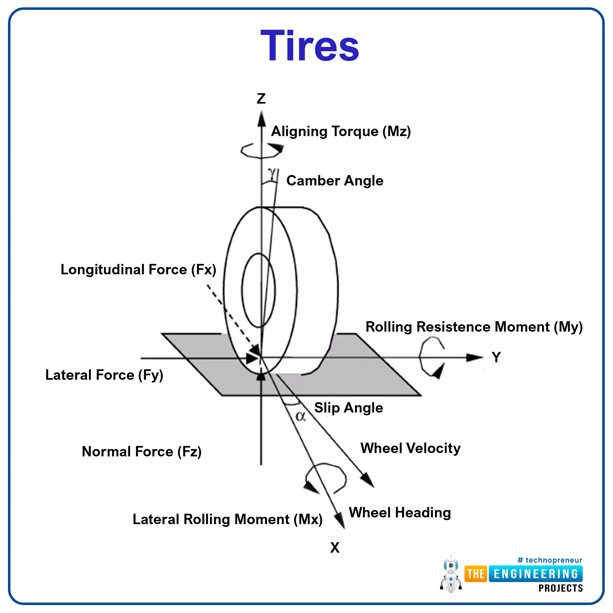
Parameters such as tire width, thread design, vehicle load on the tire define how tire behavior will be. One such parament thread design and its effect are explained below. Lateral Displacement:

Due to this behavior of pressure inside of the tire and its threaded manufacturing, the tire builds up with lateral force tire heads in an angle different than the angle at which the vehicle is leading. This difference in angle is called “Slip Angle”. This slip angle is shown as alpha in the image above.

5. Chassis

A good chassis design contributes to vehicles safety by absorbing forces during accidents. It is very important that drivers or passengers’ compartments in vehicles shall stay intent during the crash to protect them. Although from a manufacturing perspective there can be more aspects to look after, here in the study of dynamics, we enlist a few parameters of the vehicle which are defined by vehicle chassis.

Vehicle Length, vehicle width, front overhang, rear overhang, Front and rear axle center, the mass of vehicle etc. Front Over Hand is a distance from the front axle center to the front tip of the vehicle and the same for the rear overhand on the rear side.

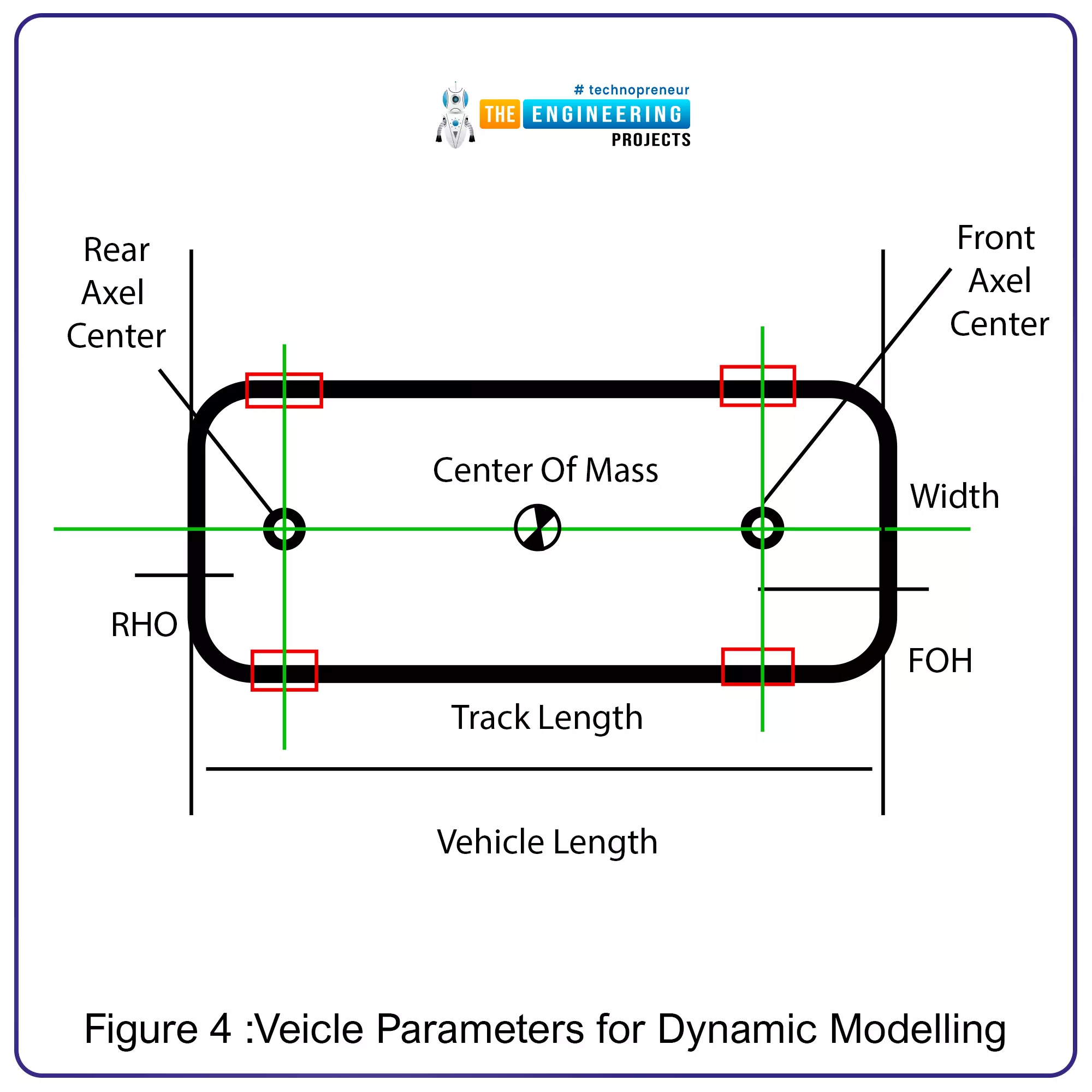
Figure 4: Vehicle Parameters for Dynamic Modelling

6. Road Dynamics

To analyze the effects of different forces on vehicles on the move it is important to understand the road model. In newtons words, the road model represents forces that the vehicle shall come across to move forward with the desired speed. These forces can be classified as

1. Forces faced by vehicle due to air
2. Forces acting on the tire: Due to friction caused between tire and road, provided friction coefficient constant of road surface and mass of vehicle we can model friction forces applied on tires of the vehicle.

Therefore, Force produced by transmission of vehicle > Air drag + Friction force for the vehicle to move in the forward direction. In upcoming blogs, we can model the road dynamics and determine the amount of acceleration required scripting these equations in MATLAB.

Figure 5: Different Road Surfaces

Verification of Models for Results

To conclude our analysis we continue programming these subsystems in MATLAB, we also need to verify the results we obtain to confirm the model efficiency and our understanding including assumptions we will make. As these prepared dynamics models fall into two categories,

1. MATLAB scripts to model the mathematical representation
2. And Simulink models to demonstrate complex concepts which may take more time to model using a script.

To validate mathematical representations writing a script to control the input variables such as desired vehicle speed or curvature will help. The flow of calling “.m” files is mentioned below:

1. load all constants and parameters
   1. run('DynamicsConstants.m');
   2. run('DynamicsParameters.m');
2. call initial condition
3. Call desired trajectory
4. Simulate model
5. Capture results and plot.

Understanding and design of vehicle model help in verification if the algorithm follows the kinematics constraint in order to make the driving experience safer and comfortable.

The second approach, the Simulink models can be validated using different inputs. One such example is to use different drive cycles to analyze the behavior of vehicles. Drive cycles contain different velocity points with respect to time. If the velocity change with respect to time is called “Modal Drive cycles”. We can conclude our analysis by observing the model’s response to these drive cycles.