Hello learners. Welcome to The Engineering Projects. We all know that matrices have been used in the engineering field for a long time, and they have a vital role in the calculation of different data. Therefore, we are learning about some very special kinds of matrices that are usually introduced to engineers at a higher level. Till now, we have seen some general operations on matrices and also examined the special kinds of matrices. Yet, today, we are moving a step forward and learning about some complex types of matrices that require strong basic concepts. So, have a glimpse at the topics that you are going to learn, and then, we’ll start practicing.

• What is a matrix?

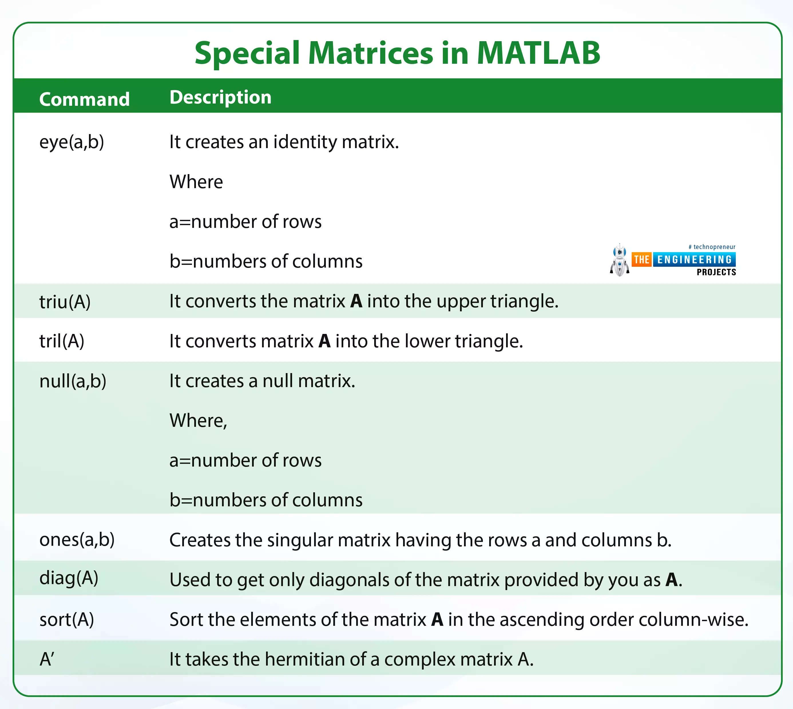
• What are the different types of matrices that are less common?

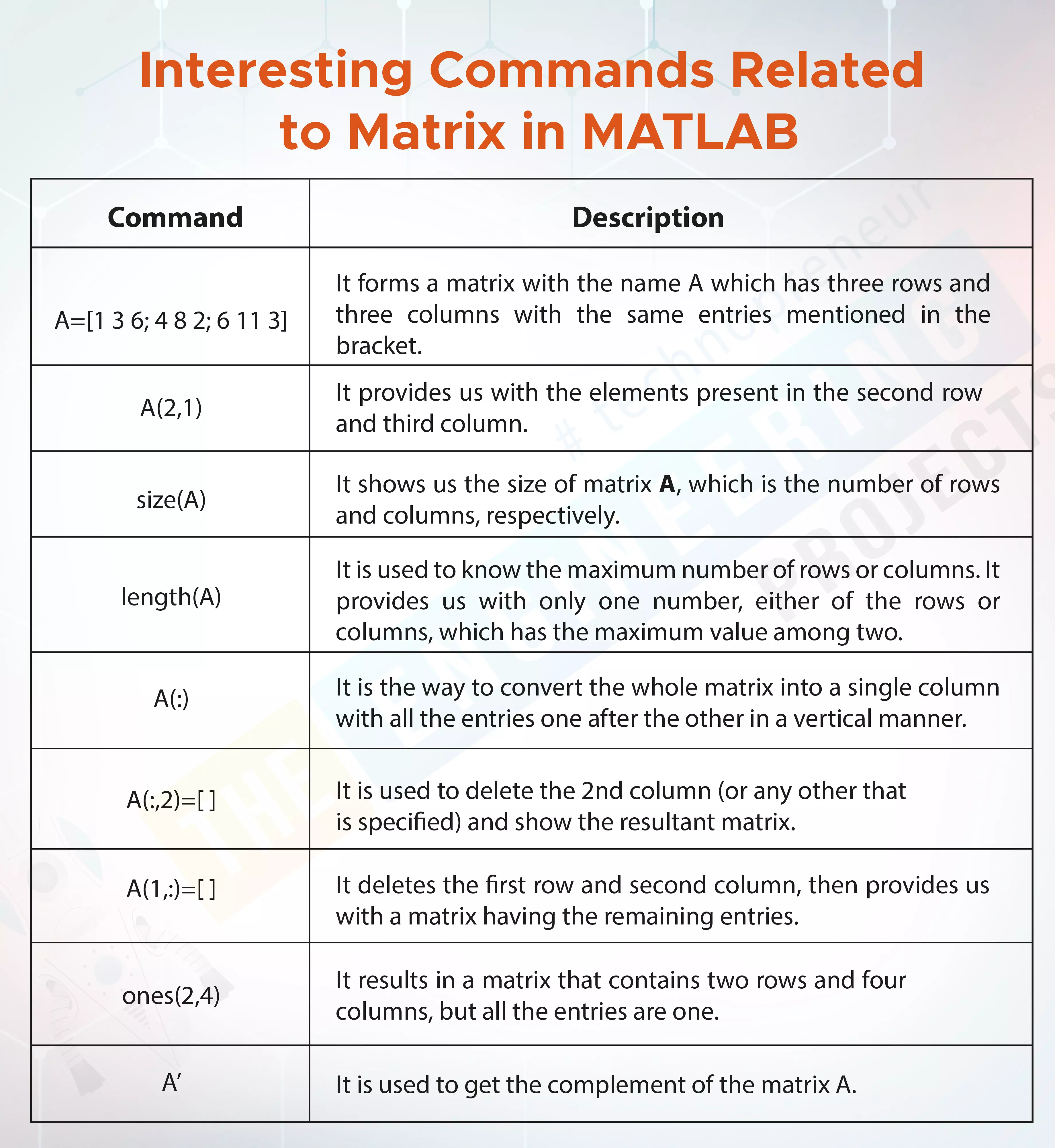
• How can we implement some interesting commands in MATLAB?

• What is the procedure for dealing with complex equations in MATLAB?

What is a Matrix?

First of all, it is recommended to learn about the introduction of the matrix. A matrix has different elements in it with different sequences, and we define it as:

“A matrix is a rectangular array in which different types of elements in the different sequences are present, and all the elements are enclosed in a long bracket that is usually a square bracket.”

The sequence and the values of the matrices are important, and the collection of horizontal lines is called a row. On the other hand, the vertical entries are collectively called columns. To find the difference in the types of matrices, it is important to know that the basic kinds of matrices are square matrix and rectangular matrix. Most of the matrices that we are going to discuss here will be square matrices. 

Types of Matrices

Depending upon different parameters in matrices, these are divided into different types and groups. In a square matrix, the numbers of rows and columns are equal to each other, and in a rectangular matrix, the numbers of rows and columns are never equal. You will observe different parameters on the basis of which these matrices are recognized, and then the behavior of each of them is examined. So have a look at these types. 

A Boolean Matrix  

We all know that boolean numbers mean two conditions only, that are, zero and one. So, the boolean matrix is the type of matrix in which only zero and one value are used, and other values are never involved. The order of the matrix may be anything, but the entries must be either zero or one.

One thing that must be kept in mind is that the matrix will surely have these values in a non-specific pattern and it never has only zero or only one. There must be one and zero of each type. We are clearing it because some other types, such as singular matrix, identity matrix, null matrix, and scalar matrix, also involve zero and one, but in a specific manner. 

Boolean numbers and conditions are used in almost every field of mathematics, and therefore, this matrix is also used in different ways in such fields. With the help of a matrix, it becomes easy to deal with a large number of data points at once. The example we have shown here has a small size. Yet, when the boolean matrix is used in practical life, we use a bulk of matrices with greater sizes. 

Orthogonal Matrices

In the previous section, we learned that a transpose of the matrix is obtained when the rows and columns, along with the entries, are interchanged with each other. Keeping this concept in mind, we can define this type of matrix as

A matrix A is called an orthogonal matrix if and only if the multiplication of the matrix A with the transpose of itself provides us with the identity matrix. 

If you are new to the identity matrix, then you must know that an identity matrix is one that contains only value 1 in its diagonal and all the entries other than the diagonal are zero. 

The inverse of a Matrix

As we have read about the orthogonal matrices, they remind us of the inverse of the matrix. It is interesting to know that there exists the inverse of a matrix that, when multiplied with the original matrix, delivers us the identity matrix. We hope you remember that an identity matrix is a type of matrix that always has the value 1 in the diagonal elements and zero in all the remaining elements. So, if we are taking matrix A, then for the inverse matrix, we can say:

A.AT= I

In this way, if we have the value of A and want to know the inverse of it, we use the following equation:

AT= I/A

So, in this way, we have observed that no matter if the inverse of the matrix is multiplied with the original matrix or vice versa, we get the identity matrix. This condition is somehow special because the multiplication of the matrix is a more complex operation than addition and subtraction, yet here we are using the rules of the dot product. There is another way to find the inverse of a matrix with the help of a formula that states that the inverse of a matrix A is equal to the determinant of matrix A with an adjoint of A. 

There are certain conditions for the existence of a square matrix:

• A matrix has the inverse only if it is a square matrix. 

• If the determinant of the matrix is equal to zero, then there is no need to find the adjoint of that matrix because the inverse does not exist for that matrix. 

It is not always necessary that in the inverse of a matrix, the values are reciprocal of the original matrix. The values may also be changed, and by dot multiplication, we can get the identity matrix.

Stochastic Matrix

Here is another interesting type of matrix in which all the values show the probability values. We know that the probability values are so small that they are less than one and have fractional values or in the form of points less than one. So, the stochastic matrix has all the probability values as its elements.

You can see all the values are less than one because the probability is usually in the form of such small numbers. If any of the values is greater, then it is not a stochastic matrix. 

Nilpotent Matrix

This is a less common type of matrix in which Ak = O, that is, for every power of the matrix, we get a null matrix (the one with all the values equal to zero). There are two conditions that must be fulfilled in this type:

1. The matrix A must be square.

2. We get a null matrix every time we apply any power to matrix A, which is a natural number.

For example, when we take the square of each value of A, we get the null matrix. It is a less common type of matrix, but at a higher level of calculations, it has its applications. 

Idemportenet Matrix

It is a type of uncommon matrix that provides us with a matrix equal to itself when any power is applied to it greater than 2. That is, An = A where the value of n is always equal to or greater than 2. Usually, it has been noticed that if the square of the matrix A is equal to itself, then there is no need to check further because the result remains the same for any number greater than 2. You can take it as homework and find examples of such matrices by yourself.

Special Commands in MATLAB

It seems like you have learned a lot about the special kinds of matrices. When we talk about MATLAB, we have observed that there are different MATLAB commands that are not related directly to the matrices yet are used to make the functioning of a group of numbers and matrices easier and more effective in some cases. So, have a look at some of the commands.

The procedure to perform the Complex Number in MATLAB

We all know about complex numbers and have also used them in the matrices when we were talking about hermitian metrics. A special kind of function in MATLAB is the “complex” function, which is used to make the complex equation. So have a look at the step-by-step procedure to perform the complex equation in MATLAB.

• Hit the start button of MATLAB. 

• Go to the command window.

• Start by writing the following command. 

a=3

w=3

• It will provide us with two numbers that we will use in the complex function. We are naming this equation ComplexEqaution, and the command to perform this is

ComplexEqaution=complex(a,w)

• Press the enter button. 

• Now, using this equation, we can also find the real and imaginary parts of the equation using different commands. For real numbers, we are writing:

real(ComplexEqaution)

• It will give us the real part of the equation. Similarly, write the following command for the imaginary number:

imag(ComplexEqaution)

• Similarly, to obtain the absolute value of the equation we have just made, we are using the required command.

abs(ComplexEqaution)

• Finally, to find the angle of the equation, we are using its command.

angle(ComplexEqaution) 

• Now, to perform the inverse of a matrix, we are going to introduce the matrix first. So, write the following command:

B=[1 55 2 7; 4 5 2 8; 4 99 1 6; 3 8 4 1]

• The command for this purpose is:

InversofMatrix= inv(B)

If you are confused about the absolute value of the complex equation, then you must realize that complex numbers are present in the plane or the coordinates of the system, and the absolute value of the complex numbers is defined as the total distance between the origin of the complex number (where the plane is (0,0)) and the complex plane (a,b). The procedure to do so is a little bit complex if we solve it theoretically, but with the help of MATLAB, this can be done with the help of a simple command and all the control in your hand. You should practice more with all these commands by using your own values in the matrix with a different sequence. Once you have followed all the instructions given above, the output at your MATLAB command window should be like the images given next:

So, in this way, we have gotten rid of the long and error-prone calculations, and by using simple commands, we have simply applied the formula of inverse, and in this way, we have not had to find the adjoint and determinant of the matrix A. 

Consequently, we had a little bit of a complex yet interesting lecture today on matrix, in which we defined it first for a solid foundation of the concept. After that, there were different types of matrices that are less common but have interesting patterns of the elements in which the values and positions are important to define the type of matrix. Moreover, we have seen some interesting commands in MATLAB to perform the operations of complex equations and also implement them all practically. In the next lecture, you are going to learn the amazing features and applications of MATLAB in different aspects of the study.

Hey students welcome to another tutorial in The Engineering Projects where we are going to learn a lot about matrices. If you are a beginner to the metrics, then you should go to learn the fundamentals of matrices. Yet, if you know the basic introduction, you are at the right lecture because we are learning about the special kinds of matrices and you are also going to see the matrices in action using MATLAB. So, here is a simple list of today’s topics. 

• What is a matrix?

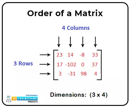
• How can we identify the matrix with the help of its general form?

• What are the different types of matrices?

• What is the concept of transpose while dealing with matrices?

• How can we implement these types of matrices in MATLAB by different commands?

What is a Matrix?

A matrix is a type of array that stores data of the same kind. It has great importance in the world of technology and it is defined as:

"A matrix takes the form of an ordered rectangular array surrounded by a square bracket and has entries of the same kind in the form of real or complex data."

To perform different operations on the matrices, you just have to apply them to the whole matrix at once; there is no need to apply them to all the entries one after the other. This will make sense when you see the matrices in action. 

Till now, we have learned about the basic introduction of the following types of matrices:

• Row matrix

• Column matric

• Square matrix

• Rectangular matrix

These are the basic types irrespective of the elements or entries present in them, and now, we are going to discuss some types that have the features of these matrices but the entries in them are in a specific pattern, so they are considered the special kinds of matrices. Before going into the details of each of them, there must be the foundation of a concept of a general form of the matrix. 

The General Form of the Matrix

To examine the location of a specific element, we use the terms "rows” and “columns” where

1. Rows are the horizontal entries of the matrix.

2. Columns are the vertical entries of the matrix.

A specific element is the part of a row and column at a time and to mention the location of an element, it is important to know the information about both of them. So, in the general form, a three-by-three matrix is shown as:

Where

• A= name of the matrix
• a= elements of the matrix A

Notice that a has two numbers with them in which the first number denotes the rows and the second one is the number of columns. To make it easier, we denote rows with i and columns with j. So we can say,

• aij=a23=element of the second row and first column

Keeping this concept in mind, now it is easy to understand the types of matrices in which the value of the elements matters. Have a look at some of these types.

Identity Matrix

The identity matrix is a special kind of matrix having the arrangement of entries in such a way that all the diagonal entries are one and the remaining ones are all zero. In this way, we get the matrix of the form:

You can observe that for an identity matrix, the elements where i=j are all ones, and all the elements other than this are zero. There are certain applications of the identity matrix and you will know them in the upcoming lectures. 

Zero or Null Matrix

Here is an interesting type of matrix. This matrix has all the entries zero and no other value can be found in this element. So we assume the zero or null matrix as:

Where the sequence of the matrix can be any. No matter whether it square, row, or rectangular matrix. 

Singular Matrix

A singular matrix is the type of square matrix that has the determinant equal to zero. It is possible in the condition when all the entries of the matrix have the value one.

We all know the procedure to find the determinant. So, taking the determinant of this matrix C, we provide ourselves with the following calculations:

|C|=1x[(1x1) - (1x1)] - 1x [(1x1)-(1x1)] + 1x[(1x1)-(1x1)]

    =1x(1-1) - 1x(1-1) + 1x(1-1)

    =1x(0) - 1x(0) + 1x(0)

    = 0 - 0 + 0

    =0

So in general, we say, in a singular matrix:

|C| =0

Non-singular Matrix

A non-singular matrix, on the other hand, has entries in such a way that the determinant is never zero. So, we can say, most of the matrices are included in a non-singular type of matrix. Here is an example of a non-singular matrix, which we have also mentioned in other categories.

|C|=3x[(-6x7) - (1x-1)] - 0x [(2x7)-(1x4)] + (-5)x[(2x-1)-(-6x4)]

    =3x(-42+1) - 0x(14-4) - 5x(-2+24)

    =1x(-41) - 0x(-10) + 5x(22)

    = -41 - 0 + 110

    =69

Hence, we can conclude for the non-singular matrix that if A is a non-singular matrix, then:

|A|≠ 0

Diagonal Matrix

The concept of diagonal was used in the identity matrix, but it is a slightly different case. A diagonal matrix is one that has all the entries, other than the diagonal, equal to zero. The values in the diagonal may be anything. 

Here, one concept must be clear. In some cases, all the diagonal values except one may be zero, but it will still be called the diagonal matrix. In other words, by changing even one of the values in the null matrix, we can convert it into the diagonal matrix. 

Scalar Matrix

A scalar matrix has all the diagonal values the same, no matter what the value is, and all other values are zero. So, in the scaler matrix, three conditions must be satisfied:

1. The values other than the diagonal are all zero. 

2. The values in the diagonal must be non-zero.

3. All the values of the diagonal are the same, no matter what the value is. 

4. The matrix is a square matrix.

If one of the conditions is not satisfied, it is not a scalar matrix. 

Upper Triangular Matrix

This is an interesting type of matrix. The upper triangular matrix can be recognized when all the entries below the diagonals are zero and the entries above the diagonal are non-zero. So we get the matrix as:

The value in the diagonal must be non-zero for at least one value. And the 

The Lower Triangular Matrix

As you can guess, the lower triangular matrix has non-zero values in the lower elements than the diagonal. The values presented in the upper portion of the diagonal are all zero. So the lower triangular matrix looks like this:

Transpose of a Matrix

This is another concept in matrices that is important to discuss here because some types of matrices depend upon it. We know that a matrix has i rows and j columns. Then, the transpose of the matrix is defined as:

The transpose of matrix A, denoted by AT , is obtained when the rows and columns of matrix A are interchanged no matter what the total number of rows and columns. 

This concept is used in different ways, and the results obtained are important. To understand well, you must know, that a rectangular matrix of order 2 by 3 will be converted into a matrix of order 2 by 3 when the transpose is applied to it. 

Symmetrix Matrix

It is a special kind of matrix that involves the procedure of transpose. A skew-symmetric matrix is one that has the arrangement of elements in such a way that applying the transposed result in the matrix that has the same entries and same order. In other words:

AT=A

So, the skew-symmetric matrix is always a square.

The Skew Symmetrix Matrix

Here is another kind of square matrix that involves the transpose, and it is slightly different from the one discussed just before. This type of matrix, after taking the transpose, results in a matrix with all the negative values. So we define this in a simple way as

AT=-A

Harmatian Matrix

A hermitian matrix involves complex numbers in it. That means some, or all the elements of a matrix A are complex numbers, and the transpose of that matrix A results in the transpose of a conjugate matrix. So, the following conditions are applied to the hermitian matrix:

• It is a square matrix.

• It involves complex numbers.

• A conjugate of the matrix is obtained. 

• The resultant matrix has the conjugate values.

The Skew Harmatian Matrix

A skew hermitian matrix, with the complex conjugate, is the one that involves the negative values of the original matrix ( the one before the transpose procedure). It will be crystal clear to you when you examine the case given below:

Special Matrices in MATLAB

Are you enjoying the different types of matrices? Matrices are fun in MATLAB, it is good practice if we attempt all these types in MATLAB. Notice that, these types follow a specific sequence. Hence, MATLAB has a special function designed for the user with the help of which, one can have all these types by simply writing some commands. But it would be helpful if you understood the commands first.

Follow the procedure given below to perform the tasks.

• Start your MATLAB software. 

• Go to the command window.

• Start typing the codes given below and get your desired matrix.

A=[ 2 7 4; 5 11 5; 3 8 23]

• Notice that we have a square matrix now. It will help us in different operations. So let’s start using different operations. 

• Write your first command.

IdentityMatrix=eye(3,3)

• It will create an identity matrix with the name IdentityMatrix with three rows and columns.

• Similarly, write the command given below:

 UpperTriangularMatrix=triu(A)

• It's time to create the lower triangular matrix. So write the command.

 LowerTriangularMatrix=tril(A)

• For the null matrix, we are going to use:

NullMatrix=null(2,5)

• For the singular matrix, we are using the following command:

SingularMatrix=ones(3,4)

• If you wish to have a diagonal matrix of A, write the command:

DiagonalOfMatrix=diag(A)

• To sort your matrix A, we are using the command given below:

SortMatrix=sort(A)

• If you want to find the hermitian of the matrix, first you have to introduce the complex matrix in MATLAB. So we are writing the following matrix:

B = [1+j; 1-j; 2-j; 1+2j]    

• Now, by simply applying the command, we can get the hermitian of this matrix.

HermitianMatrix=B’

Thus, today’s lecture was full of different types of matrices, and many of them were new to us. We began with the definition of the matrix, then we saw different types of it where the data or the elements of the matrix were important. Many of them have conditions where the order and location of the elements are important. The concept of transport in the matrix was new to us, and by using it, we explored different types. In the end, with the help of different commands in MATLAB and with the help of practice, we sharpened our concepts. There are different and interesting types of matrices, and we are going to explore all of them in our upcoming lectures.

Hey peeps, welcome to The Engineering Projects. We are talking about matrices, and if you want to learn them from scratch, you must go to the introduction to matrices in MATLAB. Today, we are learning how to perform different arithmetic operations on matrices. You will also see some interesting commands that are only applicable to the matrices. Here, it is important to notice that in MATLAB, the matrices are performed in the command window and there is no need to have the programming skills to perform them. Even if you are new to programming, you can easily perform the operations in MATLAB. We’ll discuss different basic operations on the matrices and will also perform each of them in MATLAB. Most of them are urinary operations and some of them are binary. Here is a small glimpse of today’s topics:

• What is a matrix?

• What are some basic operations of matrices?

• What is an identity matrix?

• How can we use the simple commands of MATLAB to perform complex and time-taking calculations with matrices?

An Introduction to Matrices

We all know what matrices are matrices. Yet, it is important to learn the basic definition of the matrices because this will create a map of how the basic operations on the matrices are performed. So, a matrix is defined as:

“A matrix is a two-dimensional array with entries of the same kind in the form of real or complex data, and it takes the shape of an ordered rectangular array surrounded by a square bracket.”

The thing to notice here is, that the data present in the matrices are of the same kind and therefore, we can perform a simple operation on each of the entries by simply applying it at once to the whole matrix.

Now, have a look at the basic operations on the matrices. 

Basic Operations on the Matrices

There are several operations that can be performed on the matrices. Some of them are unary operations ( those operations that require only one matrix for the application) and most of them are binary operations that require two matrices for the performance. When you observe different types of each of them, we are going through the definition of each of them, and at the end, you will also practice each of them in MATLAB. So, have a look at the definition of each of them. 

The Addition of the Matrices

Yes, as you can guess, addition is a binary function, and you need two matrices to perform the addition of the matrices. The addition of the matrix takes place when both of the matrices have the same number of rows and columns. Each entry is added to the corresponding entry of the other matrix, and in this way, we get the resultant matrix with the same number of rows and columns. 

One must keep in mind that addition is a commutative operation, which means if we have two matrices named A and B, respectively, then the addition process follows the rule given below:

A+B=B+A

All other rules are the same as the simple addition, but here, the equal number of rows and columns of the matrix is an additional rule that must be followed. 

Subtraction of the Matrices

As with the addition, the subtraction of the matrices is a binary operation, it requires the same order of both the matrices and does not follow the commutative rule. It means:

A-B!=B-A

And that makes sense. During the subtraction of B from A, the element on B at a particular location is subtracted from the element present on the corresponding entry of A. So, if the value of this particular element is less than the element subtracted from it, we get the answer in minus. Therefore, subtraction is not commutative.

Multiplication of the Matrices

The multiply operation in the matrices is somehow a little bit different from the normal multiplication. Two types of multiplication occur in the matrices:

1. Multiplying the whole matrix with a scalar

2. Multiplying two matrices 

Multiplying a single number with the whole matrix is called scalar multiplication. If we are multiplying a number k with the matrix, the multiplication of k with the matrix provides us with a resultant matrix that has each entry having the value k times more than before multiplication.

On the other hand, when two matrices are multiplied, the key point to remember is:

During the multiplication of two matrices A and B, the number of rows of matrix A must be equal to the number of columns of matrix B; otherwise, the multiplication is impossible.

Hence, if you are asked to multiply the matrices, this must be the first condition that you check. So, here is the procedure of matrix multiplication.

• Check the number of rows and columns of matrices A and B.

• Multiply each element of row 1 of matrix A with the column of matrix B. 

• Add all the results of this multiplication together. 

• Now, repeat the same procedure with the other rows of matrix A with the columns of matrix B.

• In the end, you will get the resultant matrix that has the same number of rows as matrix A. 

Therefore, the multiplication of the matrix is non-commutative and therefore we can say:

AxB!=BxA

This will be more clear when you learn the example in the next section. 

Basic Operations on Matrix in MATLAB

The solutions to the operations that we have mentioned above are time taking and require a number of steps to be followed. The same results, but in a better manner, can be obtained with the help of MATLAB. Just follow the steps to perform these operations in MATLAB. 

Fire up your MATLAB software. 

• Go to the command window.

• Start writing the following code to make a matrix A in the command window:

A=[ 2 5 8; 1 8 2; 4 6 9]

• The resultant matrix will be shown on the screen. 

• Now write the following code just below the matrix formed before:

B=[1 5 2; 4 8 9; 2 7 3]

The same result will be shown for matrix B. 

• Now, to perform the addition of matrix A and B, write the following command in the command window:

A+B

It will show the results. 

• Now write A-B. 

You will get the results. 

If you are performing all the operations according to the instructions, your screen will look like the following image:

For the multiplication of both types, there are different commands. For the scalar multiplication, we are using the simple command given next:

2*A

It will provide us with a matrix that has two times the values of matrix A.

For the multiplication of two matrices, the command A.*B is used. Here, the question arises why we are using the dot in between the A and B.  Have a look at the results of the different types of multiplication. We have mentioned the results when we used this command and a simple command of multiplication as A*B.

Both types have different results. It is because using a dot between the A and B tells the compiler that we want the multiplication of each element with the other, and in this way, the authentic procedure for the multiplication is used as we have mentioned above in the multiplication section.

Similarly, we are testing the same condition while we want the square of the matrix. We all know that a square means that each and every value is multiplied by itself. On the other hand, if we simply apply a formula to multiply value 2 with the whole matrix, we’ll get the double of each value but not the square. Let’s see this in action in MATLAB.

You can clearly examine the difference between all the values. If we want to have the square of each element of matrix A, we have to use the third command with a dot between the matrices' names.

Identity Matrix 

In the discussion in the previous lecture, when we were talking about the types of matrices, we mentioned a type called the identity matrix. It is the matrix that has the arrangement of elements in such a way that only diagonal values are 1, and all the other values in the matrix are zero. It is an interesting type of matrix, and when talking about the procedure for having an identity matrix in MATLAB, it is more interesting. The following command is used to make an identity matrix:

eye(x,y)

Where,

x=number of columns

y=numbers of rows

So basically, we are just telling the size of the matrix and MATLAB provides us with the result in a second, according to our wish. It may seem that it is a less common type of matrix, but that is not true. For many calculations, where the long and time-taking data is to be converted into a relatively simple identity matrix is used. It is also useful in systems where only binary data is used for calculations. There are some other uses of the identity matrix, but we are not going to discuss them because they are out of the scope of this lecture.

Let’s see this in MATLAB:

Interesting Commands Related to Matrix in MATLAB

MATLAB provides us with great ease in dealing with the matrices and we can use them to easily get quick and easy access to our data. So go to the command window of your MATLAB again and run the following commands on it. It's fun. To compile all the things into just one table, we have added the commands that have been discussed in the early sections of this lecture.

These are some very basic commands that are related to the information that we have provided you till now. A great number of commands are also associated with the matrices in MATLAB, and we are going to discuss most of them in our discussion, but it is not possible to cover all of them in a single lecture. 

Thus, today we learned a lot about matrices. We have observed some very basic but specific actions that are only possible when data is in the form of matrices. It was interesting to know that we could easily perform long calculations in MATLAB with the help of simple commands in no time. We have seen some interesting commands in MATLAB with detailed descriptions. We have also examined the output at each and every step. There are some other functions of MATLAB that help us get the results of complex commands in seconds. You must practice more by changing the elements or the numbers of rows and columns and check what results from you get with the same commands. In our next lecture, we have a lot of information about matrices.

Hello, learners welcome to The Engineering Projects. We are working on MATLAB, and in this tutorial, you are going to learn a lot about matrices in MATLAB. We are going to learn them from scratch, but we will avoid unnecessary details about the topic. So, without wasting time, have a look at the topics that you will learn in detail.

• What is an array?

• What is the matrix?

• How can we declare a matrix in MATLAB?

• What are the different types of matrices?

• Can we find the unknown values of two equal matrices?

• How can we solve the simultaneous equation in MATLAB?

What is an Array?

In this world of technology, the use of data is everywhere, and therefore, we can say there is a need for arrays in every field. You will find the reason soon. But before this, look at the introduction of an array.

 An array is a simple data structure that contains a collection of data presented in contiguous memory locations.

So, the term “contiguous” used in the definition tells us that the data is in a continuous format, so we are not required to search here and there because the data is in a structured format. Moreover, arrays are of many kinds, such as

• Two-dimensional arrays

• Three-dimensional arrays

In different types of cases, the suitable array is picked up so that we may get the best result with limited memory occupancy. With this type of foundation concept, we can now move forward toward our main topic, which is matrices. 

What is a Matrix?

In real-life applications and in higher studies, matrices are used in plenty in different forms, and therefore, we have decided to talk about them from a very basic level since it is important to understand the key features of the topics we are studying. Moreover, matrices are introduced in early classes, and it is important to refresh the basics in our minds so that we may proceed to the more complex problems. Here is the definition of "matrix":

A matrix is a two-dimensional array in the form of an ordered rectangular array enclosed by a square bracket that has entries of the same kind in it in the form of real or complex data.

The plural of the matrix is matrices, and sometimes the rectangular bracket is replaced by the parentheses according to the case. Just look at the image given below:

This is a matric that contains nine elements, and you can also name this matric anything you want. In this way, it becomes easy to deal with more than one matrix, and you will see this action soon.

Order of a Matrix

To proceed forward, you must know the types of matrix and, for this, it is important to know the order of the matrix.

The matrix given above is a square matrix and the horizontal lines are called columns, whereas the vertical entries are termed the rows of that particular matrix.

If we represent the rows with the name m and the columns as n, then the order of the matrix is given as:

mxn

In this way, it is clear that the matrices given above have the order 3x4. If it seems to be an unnecessary thing to you, think again, because, with the help of order, we can know the type of a matrix and then perform different types of operations on it. But before this, have a look at some code in MATLAB to design matrices of different kinds. 

Code for the Simple Matrix

The Matrix is easily used in MATLAB, and you can start working with it by following the simple steps given below:

• Start your MATLAB software.

• Go to the command window.

• Start writing the following code:

A=[23 14 -8 33; 17 -102 0 37;3 -31 98 4];

• Press enter. 

In the image given overhead, these are the same entries that we have seen in the image given above, and in MATLAB, you will see the following result:

The square bracket is not shown on the sides of the array in MATLAB. As you can see, the semicolon after every three entries indicates that the row is completed and the MATLAB compiler has to start the other row. 

Here, A shows the name of the matrix that is compulsory, and you can name your matrix any word. If you do not follow the exact format and provide the number of entries different in rows, you will get the error. Once you know how to get started, you are ready to learn about the types of matrices.

Types of Matrices

There are several different types of matrices, and you can perform different arithmetic operations on the matrices only if they are of the same kind. This condition is not applied to all the operations, but most of them follow these rules. Here are some important types of matrices.

Row Matrix

A row matrix contains only one row and it is one of the simplest forms of a matrix. In this way, we get the matrix with a horizontal shape. The order of this matrix is:

mxn=1xn

Where n may be any number. 

Column Matrix

As you can guess, the column matrix is a type of matrix containing only one column and one or multiple rows. In this way, we get a matrix that has a vertical shape. Have a look at the order of a column matrix:

mxn=mx1

Where m may be any number, but the value of n is always one.

Square Matrix

A square matrix always has the number of rows and columns equal. It means, that no matter what the total number of entries is, the number of entries in each row and column must always be equal. In other words,

m=n

When you examine the example of a square matrix, you will get the reason why it is called so. The shape of this type of matrix is always square.

Rectangular Matrix

A rectangular matrix is one that has the arrangement of elements in such a way that the number of rows of the matrix is not equal to the number of columns. The same statement can be represented in the equation given next:

m!=n

Therefore, the matrix formed is in a rectangular shape, either in vertical format or horizontal format, according to the number of rows and columns.

Diagonal Matrix

We all know that the diagonal is the line or area that joins the upper left area with the lower right area of a rectangular or square. By the same token, a diagonal matrix is the one that contains all the diagonal values equal to zero and s in such a way that all the values other than the diagonal are zero. It will be clearer when you see the example of the diagonal matrix. We have set the examples of all the types of matrices that we have defined previously into a single MATLAB screen so you may have the best idea of each of them.

Code and Output

Moreover, here you can observe that instead of naming the matrices A, B, and so on, we have used the real names of the matrices for a clear declaration. Your homework is to make examples of each of them by yourself for the sake of practicing.

Finding the Unknown Values Between Two Matrices

Do you remember when we said the order of the matrix matters? This is one of the uses of an order of a matrix. Suppose we have two matrices named A and B, declaring that both are equal. This means that each corresponding value of a matrix A at position row 1 column 1 is equal to the corresponding value of the same position of matrix B. This is true for all the remaining values q of both matrices. Let me be clear with one example. Have a look at the picture given below:

So, the value of r and, in return, the value of all r variables in each entry can be easily obtained by following the rules of the equation. It is one of the simplest examples of doing so, but in real life, we face complex problems. So, we use MATLAB for simplicity and accurate results. Have a look at the MATLAB code where we are going to show you an application of you can easily solve the simultaneous equation in MATLAB as well. 

Solving Simultaneous Equations in MATLAB

By using the property of the matrix of equality in more than one matrix, we can easily solve the simultaneous equations that are difficult and time taking if we solve them by hand. So let's see how we can declare and solve the simultaneous equation in MATLAB.

Code:

syms x y

equa1= 6*x + 9*y==13;

equa2= 9*x + 6*y==12;

[A,B]= equationsToMatrix([equa1,equa2],[x,y])

z=linsolve(A,B)

Output:

Understanding the Code

To understand this code, you have to learn the basic definition of the function we have used in the code. It is the equationsToMatrix function. 

equationsToMatrix Function

The equationsToMatrix is a pre-defined function of MATLAB that converts the linear equation into a matrix so that we can use different operations on it more efficiently. It does it in the same way as we do in real life while solving the simultaneous equation with pen and paper. There are three types of syntax if this particular function. The one that we have used has the following syntax:

[A,b] = equationsToMatrix(eqns,vars)

Here, a minimum of two equations are required and the variables have the same condition. You must keep all the functions in mind and have to follow the exact syntax. Otherwise, it will show an error.

linsolve Function in MATLAB

In MATLAB, to solve the linear equation, we use this pre-defined function as it works in two ways:

1. LU factorization with partial pivoting when in equation AB=X, A is a square. 

2. QR factorization, otherwise.

In our case, it has used the QR factorization. Now, you are able to understand the code clearly. 

• First of all, the syms sign tells MATLAB that we are defining the variables. These may be one or more. But, we wanted two variables here, and we named them x and y. 

• Now, we simply provide the values of the equation to MATLAB and store both of them into variables named equa1 and equa2 respectively. 

• The values of variables and equations are fed into the eqautionToMatrix function to convert the linear simultaneous equation into a matrix for easy solving. 

• In the end, we simply named a matrix z and told MATLAB that we wanted the value of variables x and y.

Simultaneous Equation in MATLAB: Method 2

By the same token, we can use the other method that is similar to it but the way it solves the equation is a little bit different. 

Code:

syms x y

equa1= 6*x + 9*y==13;

equa2= 9*x + 6*y==12;sol=solve([equa1,equa2],[x,y])

asol=sol.x

 bsol=sol.y

Output:

Here, the only pone this is to understand. sol.x and sol.y are the functions that are used by the compiler to find the value of variables x and y respectively. You can use any variable with this sol function, after naming them at the beginning. After that, a variable is used to store and present the value of the answer obtained.

It was an interesting lecture about the matrix, and we worked a lot from scratch to the end on many topics. We have defined the arrays and seen the introduction of the matrix. We also found information about the types of matrices. Once we have a grip on the basics, we learn that a matrix can be used to find the unknown value of two matrices, and as an application of this method, we found the values of the variable by using linear equations and learned how to declare, use, and solve the linear equation with the help of matrices in MATLAB.

Hello readers, Welcome to another tutorial about the signal and system. In this lecture, you are going to read details about the ramp response of a signal. In the past lectures, we have been dealing with different types of responses of LTI systems, and therefore, we know that linear invariant systems, or LTI systems, are those which follow the rules of linearity and are also time-invariant. So, at present, our focus is to examine what happens when the ramp signals are fed into the LTI system and which type of output signal we receive. Here is a glimpse at today’s topic that we will learn deeply.

• What is the RAMP signal?

• How can you define the ramp response?

• How to use the ramp function in MATLAB to get the ramp response?

• What are some important properties of the ramp function?

• How is ramp response used in different fields in different ways?

What is a Ramp Signal?

We all know that a signal is a function of one or more variables that are independent and contain some information in them. When talking about ramp signals, we get the following definition:

“A ramp signal is the one that always has its initial condition at 𝑡  = 0,  and with time, this signal increases exponentially. Therefore, it is linear in its behavior with time.“

So, when representing these with the help of graphs, we get a smooth result all the time instead of any abrupt change in the pictorial representation. 

As with other types of signals, ramp signals can also be described in two ways:

• Continuous-time signal

• Discrete-time signals

When the ramp signal is in the form of continuous values, we represent them as:

r(t)= { t for t=>0 } and {0 for t<0}

Similarly, the same condition in the discrete-time format is described as

r(n)= { n for n=>0 } and {0 for n<0}

Let us clarify the meaning of the statements given above. In both cases, the value of t or n increases with time simultaneously. Therefore, we get the smooth slop in the case of continuous signals and smooth points when we are dealing with discrete ramp signals. In other words, the values on the x-axis and the y-axis for a ramp signal are always equal if we are plotting a graph for them.

What is the Ramp Response?

As we have discussed at the beginning of this lecture, linear time-invariant systems have the linearity property, and you can use the ramp function in the time-invariant system. It has the input at one end, then the input faces some procedures according to the conditions, and from the other side of this LTI system, we get the output. So, in simple words, we define the ramp response as:

“The ramp response is one of the responses of the LTI system when the signal used as input is the ramp signal and the output of that system has the same features.”

In some places, the ramp function is defined in other ways, but the basic definition remains the same as we have provided you before. Other ways to introduce the ramp function are:

The resultant value is when the mean is calculated between the independent variable and its absolute value, which is called the ramp response.

R(x)=(x+|x|)/2

Here,

R= ramp function 

x = the variable based on which R is taken.

Ramp Response in MATLAB

Code:

num=[0.9 0.18 0.27];

den=[1 0.2 0.3 0.4];

n=0:0.1:7;

x=n.*(n>=0);

y=filter(num,den,x);

stem(n,y)

xlabel('n /The Engineering Projects.com')

ylabel('amplitude')

grid on

title('Ramp Response in CT') 

Output:

We have used the filter function in the previous tutorials as well. But, for a revision, it is important to know about it again. 

Filter Function in MATLAB

The filter function is used when the digital filters are to be applied to a vector in MATLAB. The information that is to be fed into this function is delayed before this function. The syntax is given as

filter(b,a,x)

Where

b=co-efficient of the numerator

a=co-efficient of the denominator,

And x is different in different conditions. 

• Filter returns the filtered data as a vector with the same size as x if x is a vector.

• The filter operates along the first dimension of a matrix if x is one, and it returns the filtered data for each column.

• If x is a multi-dimensional array, the filter operates along the first dimension of the array whose size is not 1.

In our case, num and den are the matrices. So we are using the second case.

Explaining Code for Ramp Response

Have you seen the code? For a super easy-to-understand, we are going to discuss every step in detail. 

• In the first step, we declared two arrays and stored their values in the num and den separately. 

• In the second step, the time is provided to MATLAB, which shows the time has an upper limit of seven and a lower limit of zero. The interval between the times is taken as 0.1.

•  Now, we have just used these two arrays for the multiplication and used the dot along with the multiplication sign so the compiler may understand that it has to multiply every term in the loop. 

• In the next step, we are going to use all the results in the filter function, and this is the step that provides us with the results in a better manner. 

• The results are then fed into the variable y. 

• In the end, to get the result graphically, we used the stem function and provided the values of n as time. 

Note:

If you want to have the same graph in the continuous-time signal, you just have to:

1. Replace the n with t for the best representation.

2. Replace the stem function with the plot function.

In this way, you will get the same graph, but the slope will be smooth. 

Properties of the Ramp Function

To deal with different types of cases when using ramp response, one must know the properties of ramp response in detail to avoid the long calculation all the time. So here are some of these:

Laplace Transform of Ramp Response

The Laplace transform is used to convert the system from the time domain to the frequency domain, and when talking about the ramp function, it says that the Laplace transform of a ramp function results in a calculation that is equal to the square of the variable based on which the integration of that ramp response occurs.

Observe that this property is valid for the single-sided Laplace transform. 

Fourier Transform of the Ramp Function

The Fourier transform is another way to convert the function from the time domain to the frequency domain so that it may become easy to deal with that particular function. The process of Fourier transform on the ramp function provides us with the following results:

Non-Negative Nature of Ramp Function

At the start, we mentioned that the ramp function does not exist in negative values and that the values are always in positive coordinates. So, we can represent this property mathematically as

∀ x ∈ R: R(x)>=0

In this way, the definition and nature of the ramp response are now clearer in our minds. There are certain conditions when the negative values of the ramp function and in return, ramp response are obtained. In such conditions, the negative values are always ignored.

Derivative of Ramp Function

To know about this property, you must know about the Heaviside step function. It is the type of step function that always has a zero for negative values and one for positive values. It is usually denoted with a capital H. When we take the derivative of the ramp function, we get the Heaviside step function. When writing it mathematically, we get the following equation:

R’(x)= H(x)          for x !=0

There are different conditions and properties of the Heaviside step function, but we are not going to explain them because it is out of the scope of this lecture. For now, you just have to remember the equation that we discussed just before this paragraph. 

Applications of Ramp Response

We know the signals are important in almost every type of field of science and therefore, we have the emphasis learning more and more about them. When the topic is ramp response, there are different ways in which ramp signals are used, and therefore, ramp response also has an application in that particular field. So let’s discuss the important fields where ramp function and, in return, ramp response are used. 

System Testing using Ramp Response

We know that in the ramp function, the values on the x-axis are equal to the y-axis and these are always positive values. Therefore, we can guess the results before the time. This property is easily used in different systems for testing different conditions or when starting a new system, it is used to check particular features. 

Ramp Response in Engineering Fields 

In different engineering fields, signals are used in different ways, as we are learning in one such subject, “Signal and System”. Electrical, computer, civil, and other engineering disciplines involve the use of ramp signals and ramp responses. 

Ramp Response in the Filed of Finance 

Those who belong to the field of finance know that the payoff of the call option is in the form of a ramp function, and therefore, ramp response has major usage in this field. The put option is set by flipping the ramp horizontally, and the short option is obtained when the ramp is flipped vertically. The graph formed in this way is called the "hockey stick" because of its shape. 

It becomes easy to deal with the results, and we get accuracy.

Using Ramp Response in Statistics

When we use the ramp function, we face different conditions while studying statistics. Some cases are

• Multivariate Adaptive Regression Splines or MARS

• Hinge Function

To deal with such complex calculations, it becomes easy to use the ramp properties so that unnecessary work may be ignored. For example, the non-negative property of the ramp function provides us the facility to ignore the negative values and focus on the calculations of positive values. 

Traffic Signaling and Ramp Response

It may look unusual, but the real-time application of the ramp function is in the traffic signals. A bottleneck is a situation when on the highway several vehicles are entered in an unmarred way and it results in the blockage of traffic. A ramp signal is used to break up this blockage, which is a cost-effective way to deal with this situation. The work is done. When the ramp signal is applied to the traffic lights effectively, this is one of the easiest ways to deal with this situation.

Today, we learned a lot about the ramp response, ramp function, and unit ramp signal. We saw the introduction of all of these and the interesting thing about the ramp response was the code of the ramp response in MATLAB because it was so clean and easy to understand. In addition to this, we have learned about some properties of the ramp function that helped us to clear the concepts and to know how we can skip long calculations all the time if we know the properties of the ramp function. In the end, we had a glance at the application of the ramp function in different fields of science, such as statistics, engineering, and finance. We hope it was an informative lecture for you. Stay with us for more interesting lectures about signals and systems.

Hey readers, welcome to another interesting lecture of this series in which we are studying signals and systems. In the present lectures, we are learning the details about the responses of LTI systems, and today, you are going to learn the step response. We also talked about the impulse response and frequency response, and therefore, this lecture will be easy for you to understand because it is, somehow, related to the impulse response. If you are new to this concept, do not worry because there will be a revision of important points side by side. Have a look at the list of today’s concepts:

• What is an LTI system?

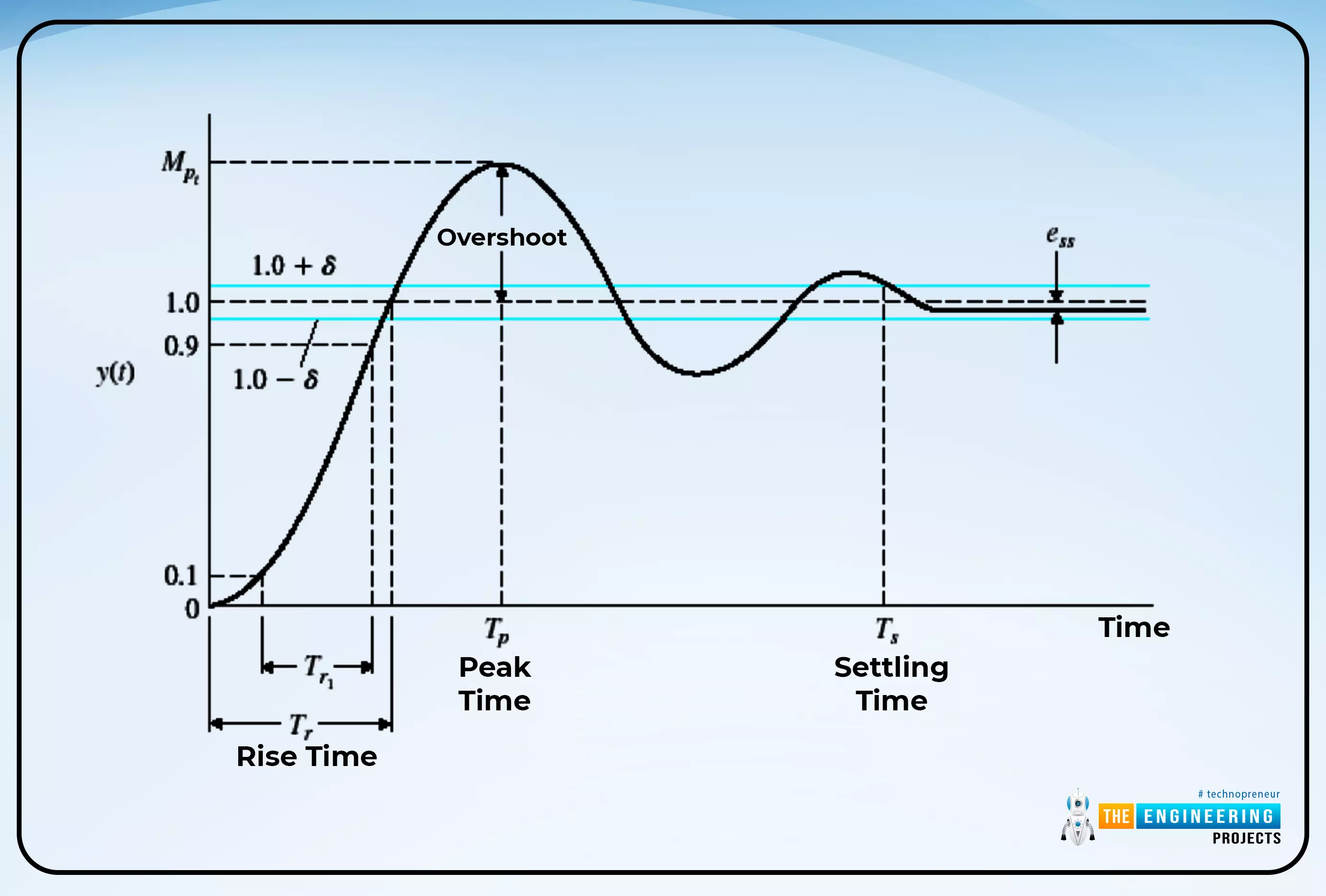
• How do you define the step response of an LTI system?

• What is the code to run the step response of signal in MATLAB using different functions?

• How can you find the detail of the graph of the step response?

• What is the difference between step response and impulse response?

We are going to learn each of them in detail so that if you know any of these already, you may have a revision about the topic.

What is the LTI System?

We all understand that a system is something that receives input at one end and produces output at the other end after performing specific operations on the input. We define the LTI system as follows when discussing it:

The term "linear time-invariant system," or "LTI system," refers to a system that simultaneously possesses both linearity and the time-invariant property.

So, keeping this in mind, we are going to discuss the whole concept of a step response in the LTI system. Refresh the definition of convolution in your mind so that it says convolution is the process in which two signals are overlapped in such a way that they form a third signal. So, keeping in mind the above image, we can use this concept to define the step response of the LTI system. 

What is the Step Response of the LTI System? 

First of all, let us clear that step signals are the one whose values always lies in just positive time and for the negative time, these signals does not have any value. The unit step signals are usually denoted as u(t). So, mathematically, we can say the step step signals are formed with the value only when t> = 0, and for t<0, signals do not exist. In this way, we get the signal at the right area of the graph, that is, the positive side values of the time. By the same token, the step response is the behavior of the LTI system when the input is provided in the form of a step signal and the output then depends upon the integral of the impulse response of that LTI system. We’ll see the proof of this statement in just a bit, but prior to that, have a look at the definition of step response:

“The step response of an LTI system is obtained when the input provided to the system is unit step and, therefore, the output also has similar characteristics.”

Using all this information, we can derive the formula for step response:

s(t)=h(t)∗u(t)

Where:

s(t)= step response

h(t) = impulse response

u(t)=unti step response 

Then,

S(t) = H(t). U(t)

S(t)=(1/t).U(t)

Now, applying the inverse Laplace transform to the equation given above, we get:

s(t)=∫h(t).d(t)

So this is the final formula that is used to calculate the value of the unit step function in an LTI system. You must know that here h(t) is the impulse response of the system that we also have read in detail in the previous session. You can have stronger concepts if you examine the example that we are going to discuss in the next section. 

Step Response in MATLAB

Code

num=[9];

den=[6 1 8 7];

a=tf(num,den);

step(a,0:0.1:8)

xlabel('n /The Engineering Projects.com')

ylabel('amplitude')

grid on

title('Step Response of LTI System') 

Output:

There are some functions that are used here but are new to you. So, have a look at the details of each of them and then try to understand the code.

The Transfer Function in MATLAB

It is an important function in MATLAB that gives us the facility to have the same results by using this function instead of using many lines of code. Using this function, we can represent the numerator and denominator in polynomial form. The syntax of this function is

y=tf(num, den)

where num and den are specified before using this function. These are the numerator and denominator in descending power of s and are in the form of a polynomial. For example, in the code given above, the equation we used is

9/6(s)^3+1(s)^2+8s+7

Before the introduction of this function in this series, we used different and relatively complex calculations in the code to achieve the same results. In short, this function has made our work simpler. 

Step Function in MATLAB

MATLAB has a built-in function step that is used to get the step response of an LTI system. The syntax of the step function is given as:

step(x,y)

Where 

x = the equation whose step function is required.

y = the time interval of the step function.

Usually, the equation is in the form of a polynomial and it is pre-defined when this function is called. You can also use the variable in which the time interval is stored before using it. Yet, we have used the exact time interval so that you may have the concept of doing so. 

How the Program of Step Response Worked at MATLAB

• First of all, we have declared the values of the polynomials of the numerator and denominator and stored them in the variables num and den, respectively. 

• We have used the transfer function to convert these values into a polynomial equation and then saved the result into the variable a to use later. 

• Next, we used the step function and put all the required values in it. 

• Notice that we have not used the stem or plot function to represent the results in the graphical format. We have just used the labels on the graph. It means the step function itself provides you with the information in a graphical format. 

• Another thing to notice is the visibility of the text “Second” on the time axis of the graph. We have not used it in the x-label but it is automatically defined in the step function. 

How to Examine Step Response in MATLAB

Here is an interesting thing about the step response. You can directly examine the graph by following some simple steps. 

• Write the code in the editor window. 

• Run the code

• Provide the path and save the program. 

• A graph will appear as shown in the code given above. 

• To examine it clearly, left click on the graph. 

• Different options will appear on the screen. Hover the mouse over the characteristics. 

• You can tick the feature on the graph you want and can choose more than one at a time. 

• Once you follow the step given above, you will get the details according to the graph. A great overview of the graph is given in the image given below:

Let’s understand what is going on the each step and why these terms are labeled so. 

Overshoot

In the graph of step response, overshoot is the area that shows the highest bump in the graph. Basically, it shows that values that are shot over the targeted values, which is why it is named so. At its start, the values indicate the values are exceeded to their steady state and at their end, the values indicate the transition from different values. 

Rise Time of Step Response

The rise time in the graph of the step response is the area that indicates the time required by the step response to reach 10%-90% of the final value to bring the system to a condition called overdamped. It also indicates the time limit when the system takes the time to reach 0%-100% to meet the underdamped condition. 

Peak Time of Step Response

The peak time of the step response is the specific value of time in the graph of step response when the overall response of the system reaches its maximum position. Usually, you can see that it is the peak value of the graph. 

The Settling Time of Step Response

The response's settling time is the amount of time needed to calm oscillations and maintain a 2% to 5% error (or tolerance) band from its final value.

So, in this way, you can understand what is going on in the step response. It is a common question how the step response is different from the impulse response because the basics of both of them are similar and why do we find both of them in the signal? 

Difference Between Step and Impulse Response

Many times, when dealing with the signal, people are confused between these two because of the similarity in the system and some other resembling features. Therefore, we have made a comparison between these two, and here are some important points about them.

Why Do We Use Step Response in LTI Systems?

There are several cases where it is more useful to have the step response over the other types of response. Some of the major reasons are listed below:

1. The step response is used because it does not require information about the dynamics of the system; hence, it can be run with the help of less information. 

2. If we have the values of the step response, we can find the impulse response by simply differentiating the step response. In this way, we can solve the system even if we do not know the initial condition. 

3. It is important to notice that integration has noise rejection characteristics, and we have discussed before that step response is the inherited integral of the impulse response. 

In this lecture today, we have read a large piece of information about the step response. To have a solid foundation for the topic, we have to refresh the concept of the linear time-invariant system and the step signal in our minds. Moreover, we have also seen the example of step response in MATLAB. For a clear idea, we also read a detailed description of each function used in the code, and then we read about the flow of the program in MATLAB. In the end, we read the details of different terms used during the examination of step response and also differentiate between step response and impulse response. In the next lecture, we will learn more about MATLAB and signals. To learn more, be with us. Till then, have a nice day.

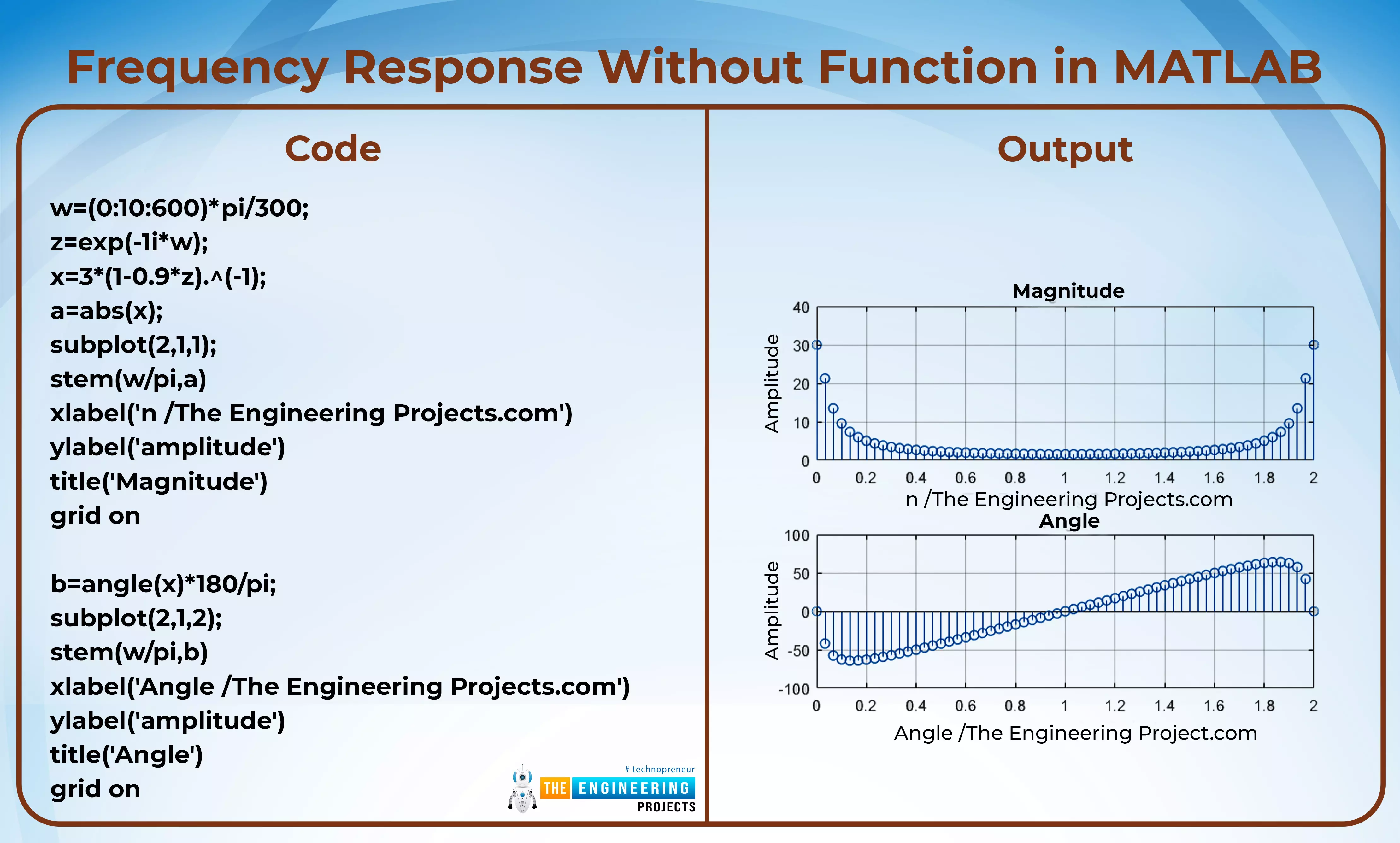
Hello learners, Welcome to another tutorial on signals and systems. We are learning about the responses of the signals. We all have experience in situations where the change in the frequency of a system, such as radios or control systems, results in a change in the working or result of that system. So we have the idea that frequencies play an important role in different types of systems. In the previous lecture, we saw the impulse response of the system. Our mission today is to learn about the frequency response of the LTI system. We will learn all the basic information about the topic and will revise some important points as well. To do this, have a look at today’s concepts:

• What is the LTI system?

• What is frequency response?

• How is frequency response performed without the function in MATLAB?

• How is frequency response performed in MATLAB by using the function?

• What are the applications of frequency response in other fields?

What is the LTI System?

We all know that a system is something that has input at one end and, after certain procedures on the input, the output is obtained from the other end. When talking about the LTI system, we define it as:

“The linear time-invariant system, also known as an LTI system, is one that possesses both linearity and the time-invariant property simultaneously."

Now, to make a solid foundation, let's recall that a signal is represented in the form of a wave, and all the waves are made of three basic quantities:

1. Magnitude

2. Phase

3. Frequency

The time period of the wave is the inverse of frequency, and in this way, if we know the magnitude (amplitude is used interchangeably), frequency, and phases, we can form a wave or signal. 

The Frequency Response of the LTI System

We are using discrete-time signals to learn the frequency response of the LTI system. The frequency response is the steady output of the system when the input is in the form of a sinusoidal signal. Before going into the proper definition of frequency response, you must know about the types of responses in the system. 

Types of Responses in the System

Responses are the types of behavior or results that a system represents. There are two types of responses in the LTI systems:

1. Transient response

2. Steady-state response

The details of both of these are not necessary here. To make it simple, we are not discussing the transient response here. 

Introduction to Frequency Response of the LTI System

As we have read a little bit about this function, we know the type of response we are discussing. You must know that frequency is the steady-state response of the system, which means the frequency repose tells us how the system will work in the steady state.

The frequency response of the LTI system is a type of steady response, and both input and output are in the form of sinusoidal waves with the same frequency but with different values of amplitude and phase angle.

r(t)=Asin(ω0)              (eq. 1)

Similarly,

G(s)=G(jω)                 (eq. 2)

If we represent the equation 2 in the form of phase and amplitude. then,

G(jω)=|G(jω)|∠G(jω)

Replacing ω with ω0 we get,

c(t)=A|G(jω0)|sin(ω0t+∠G(jω0))

So, by using these equations, one can calculate the magnitude and phase of the wave through frequency response.

If you have the idea of impulse response that we have discussed in the previous lecture, then you must have an idea of how the LTI systems work. Yet, in the case of frequency response, we are going to study it in another way. It is now time to discuss some examples in which we will get the different procedures to perform the frequency response efficiently in MATLAB.

Frequency Response Without Function in MATLAB

Code:

w=(0:10:600)*pi/300;

z=exp(-1i*w); 

x=3*(1-0.9*z).^(-1);

a=abs(x);

subplot(2,1,1);

stem(w/pi,a) 

xlabel('n /The Engineering Projects.com')

ylabel('amplitude')

title('Magnitude')

grid on

b=angle(x)*180/pi;

subplot(2,1,2);

stem(w/pi,b) 

xlabel('Angle /The Engineering Projects.com')

ylabel('amplitude') 

title('Angle')

grid on

Output:

We have used a new function here, and we want to discuss it before elaborating on the program given above.

Angle of the Wave through the Function in MATLAB

To find the angle at which the wave or, in return, a signal is working, we use the following function:

angle(x)

This function calculates the angle of the wave whose value is stored in x and, after that, using the stem function of results, provides us with the resultant wave. Now let’s move toward the code and match the statements given next with the code.

• It is a simple program that uses some basic operations. We are using these operations in a different way to get the output of the frequency response. Let’s discuss what happened in this code.

• First of all, we have provided the value of omega. Here, time is represented in a simple way, as we have been doing it from the beginning so far in this series. Yet, multiplying the whole time period t with pi provides us with the value of omega. 

• This value is used in the exponential form while it is being multiplied with the imaginary number. So, we are providing a variable z in which the whole value of the is saved. 

• This is used to provide the equation that we want to work with. 

• Once we get the equation, we are then using the absolute value of this signal and plotting it on the y-axis where the time period is on the x-axis as always. 

• To get the angle of the wave, we are multiplying the angle results by 180 degrees and simply representing the data in the form of a discrete value graph. 

Frequency Response Using Built-in Functions

Code:

a=-4*pi:0.4:pi;

num=[7 1] ;

den=[1 -0.32] ;

h=freqz(num,den,a); 

subplot(2,2,1); 

stem(a/pi,real(h)) 

xlabel('n /The Engineering Projects.com')

ylabel('amplitude')

grid on

title('Real Part')

subplot(2,2,2); 

stem(a/pi,imag(h)) 

xlabel('n /The Engineering Projects.com')

ylabel('amplitude')

grid on

title('Imaginary Part')

subplot(2,2,3); 

stem(a/pi,abs(h)) 

xlabel('n /The Engineering Projects.com')

ylabel('amplitude')

grid on

title('Magnitude')

subplot(2,2,4);

stem(a/pi,angle(h))

xlabel('n /The Engineering Projects.com')

ylabel('amplitude')

grid on 

title('Angle')

Output:

We have used some built-in functions of MATLAB here, and the description of all of them is here:

Real value Function in MATLAB

This is an interesting function that takes a signal or wave and provides us with the value of the real part of the wave by ignoring the imaginary part containing values of iota and other imaginary numbers. You just have to feed the value of a signal into it. The syntax of this function is

real(x)

where x is any signal. 

Imaginary Value Function in MATLAB

Yes, you are guessing right. This is the function used to get only the imaginary part of the wave, and the real-time values are ignored with this function.

imag(x)

Here, x is the number/signal, and you just have to put the results into this function. 

Let’s understand the code now.

• At the beginning of this code, we provided the time period and stored it in the variable a. We used the variable t for this purpose, but I just want to show that it's just a variable and you can name it anything.

• After that, we provided the information for our equation and then fed it into the built-in function of frequency response to get the results. 

• In the end, the results are shown with the help of a graph for better representation. 

• The equation provided by us had different parts, and for the best understanding of the concepts, we used each part of the signal and shown it in the form of a separate signal. 

• In the second part of the code, we are using the stem operation, in which we use the time period on the x-axis and the imaginary part of the resultant signal on the y-axis. 

• We all know that magnitude is the absolute value of some wave, and here, we are using the absolute function to represent the magnitude. We have also used this function in the other codes in this series. 

• The last part contains the angle of this wave, and we have used the angle function here. In this way, the changing angles of the wave throughout this procedure are shown on the graph with the help of stem operation. 

Frequency Response Using Fast Fourier Transform

Let’s try to use some of the concepts of the signal and system that we have learned till now to calculate the frequency response in another way. 

In the previous lectures, we have said that the transforms are used to convert the signal from the time domain into the frequency domain. We are using this concept and converting the frequency domain, and in return, we are simply presenting the signal in graphical form. For this, let’s try the shortest method, which is the Fast Fourier transform, and to make it simpler, we will use the built-in function in the code. All these concepts are used in the code given below, so have a look at them. 

Code:

signal=[11 44 12 27 53 19 34 ];

a=fft(signal);

subplot(2,1,1);

stem(signal,a)

xlabel('n /The Engineering Projects.com')

ylabel('amplitude')

grid on

title('(n,fft(n))')

subplot(2,1,2);

stem(a);

xlabel('n /The Engineering Projects.com')

ylabel('amplitude')

grid on

title('(fft(n))')

Output:

Here you can clearly see that we have provided you with the two types of signals. One has the time on the x-axis and the frequency part on the y-axis. On the other hand, the second wave represents the frequency part of the wave only. 

Application of Frequency Response

As you can see in the information given above, frequency response is the measure of the magnitude and phase of the signals in the LTI system. There are several applications of frequency response, and some of them with their details are given below:

Frequency Response in Sound Systems

We all have experienced the role of frequency in sound devices, especially in the music system, where changing the frequency of the sound system results in a change in the quality of voice and some other features. Frequency response evaluates whether and how well an audio component reproduces each of these audible frequencies, as well as whether it modifies the signal along the way.

Radio Spectrum Frequency Response

There are certain frequencies that come in different regions and using these regions results in interesting applications. Changing in the frequency spectrum results in the usage of frequency response in the field of different cables, such as

• Video switching

• Twister pair cable

• Coaxial cables, 

and some other types as well. 

When changing the radio spectrum of the cables results in a change in the behavior of the cables in working condition and the data rate and other features.

Reading the Waves Through Frequency

Frequencies are used in different ways to measure the infrasonic frequency response. We have seen that the prediction of earthquakes in the past was done with the help of the change in frequencies of waves. Moreover, some specific types of waves are used in the diagnostic and working of brain waves. In this way, frequencies are used in the medical field as well.

Today we read about the frequency response and worked in MATLAB to get the concept through the practical implementation of the signals. In digital systems, frequency response is an important concept, and we have seen its multiple applications in different fields. These are just the introduction and when studied deeply, they can be used in complex systems efficiently. Get ready for other topics related to signals and systems that we are going to discuss with you soon. As for homework, you must practice more and more on these topics and try to solve the problems.  Examples are given in MATLAB theoretically by your own research and match the result to whether you get the same results when trying the theoretical procedures.

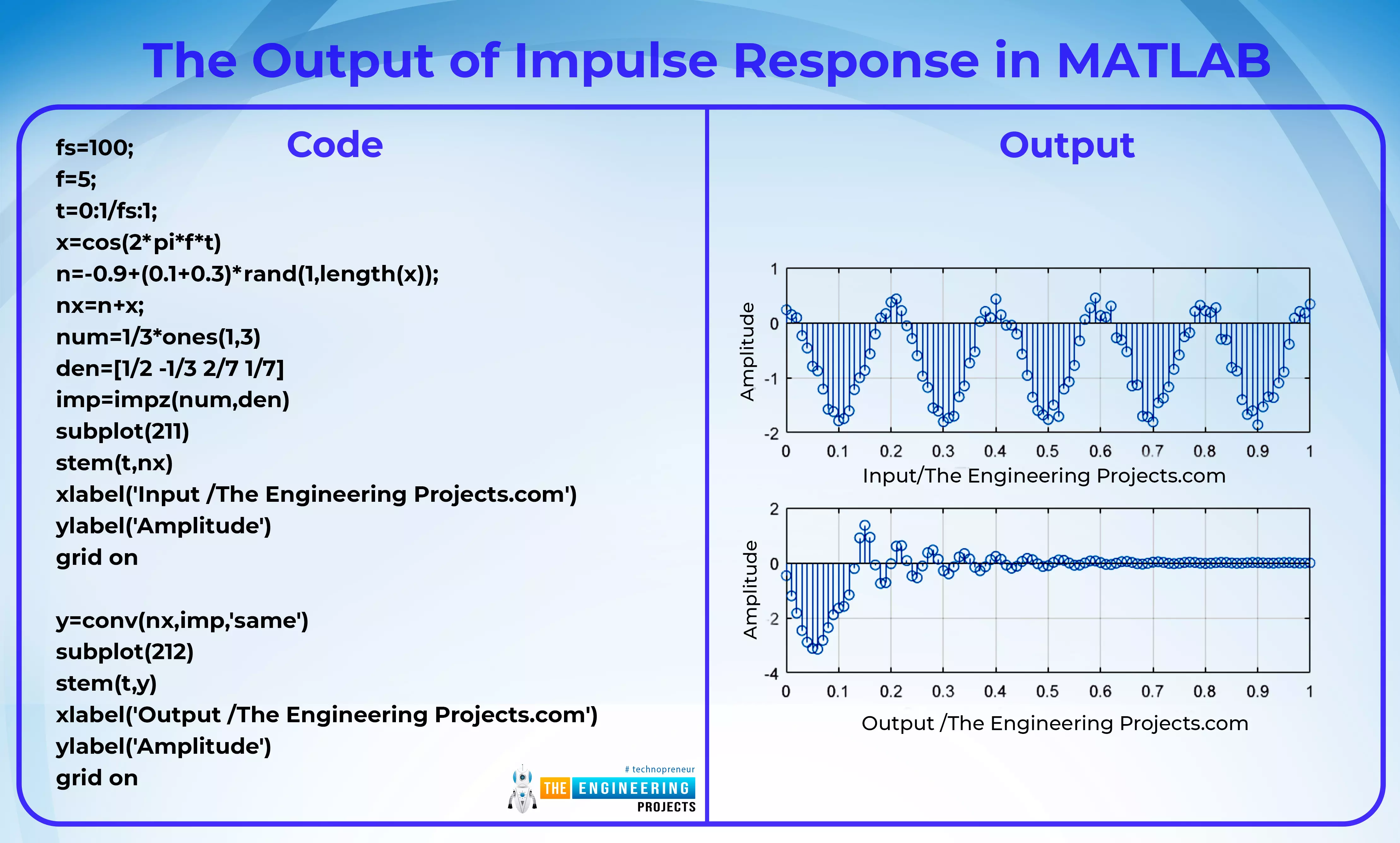
Hello learners, welcome to another topic of signals and systems. We hope you are having a reproductive day and to add more information in the simplest way to your day, we are discussing the responses in discrete-time signals. If you do not get the idea of the topic at the moment, do not worry because we are going to learn it in detail and you are going to enjoy it because we are making interesting patterns in MATLAB as the practical implementation of the topics. Have a look at the points that we are making clear today. 

• What is the LTI system?

• What is impulse response?

• How can we get the impulse response in MATLAB?

• How can we have the output signal using codes and impulse response in MATLAB?

As we have learned so far in this series, there are two types of signals based on the shape of the signal we obtain, and these are

1. Discrete-time signals

2. Continuous-time signals

The focus of our topic is discrete-time signals in which the points of the signals are not connected with each other, but we get a line for each point in the graph, and in this way, we get a non-continuous wave. There are different types of operations that can be performed on discrete-time signals to get useful results from them. The types of operations that we are going to discuss on discrete-time signals are

1. Impulse Response

2. Frequency Response

Both of them are simple yet different from each other, and we are going to discuss all the necessary details about the impulse response in the next section. But to make a solid foundation, let us first define the LTI system. 

What is an LTI System?

We have read about the types of systems at the beginning of this course, and we know that:

“The LTI system, or the linear time-invariant system, is those which have both characteristics at the same time, that is linearity and the time-invariant property."

We are now moving towards the introduction of the impulse response.

Impulse Response in DT Signals

Recalls that a system is something in which we provide the input at one end of the system, the operations in the system take place on the input, and from the other end of the system, we get the output. 

Now coming towards the impulse response, it is the procedure or the operation that is implemented on the discrete time signal and after the application of this signal, we get the required output. To clarify this statement, have a look at the image given below:

The impulse response here is the procedure that converts the input into the required output. When calculating the result theoretically, we use the mathematical form of this image. 

x[t]=h[t] * y[t]

Considering the equation given above, we see that it is in the form of a time domain, and if we want to change it into a frequency domain, then we are using the Laplace transform (if you don't know it, recollect from the previous lectures).

L(x[t])=(h[t] * y[t])

Y(s) =X(s). H(s)

And in this way, we can also change the form of the equation to get the required quantity. 

Y(s) =X(s). H(s)

Or

H(s)=Y(s)/X(s)

So, in this way, we can calculate the impulse response of the discrete-time signals. The H(s) here is called the transfer function, and these are used interchangeably. When we use the function in the time domain, we call it an impulse response, and in the case of the s-domain, we call it the ratio of input and output transfer function. Both of these are used for the LTI system.

While performing the transform, the signal from the time domain to the frequency domain, you can also use the other forms of transforms as well, if you do not want to use the Laplace transform. The other two types of transform that we already know are

1. Z transform

2. Fourier transform

Impulse Response in MATLAB

Once you know the basic definition of the impulse response, you might be interested in the example. We are describing the two methods to perform the impulse response and instead of making two different programs, we are merging them into one. Suppose we want to perform the impulse response operation with the equation given below:

½(y[n]-⅓[y-1]+2/7[y-2]+1/7[y-3]=(x[t]+x[x-1]+x[x-2])/6

Have a look at the program and if it confusing for you at the moment, do not worry, we are going to discuss it in just a bit. 

Code:

fs=25;

t=0:1/fs:1;

c=(t==0)

num=1/3*ones(1,3)

den=[1/2 -1/3 2/7 1/7]

y1=filter(num,den,c)

subplot(211)

stem(t,y1)

xlabel('Using filter method /The Engineering Projects.com')

ylabel('Amplitude')

grid on

y2=impz(num,den,length(t),fs)

subplot(212)

stem(t,y2)

xlabel('Using impulse Function /The Engineering Projects.com')

ylabel('Amplitude')

grid on

Output:

Filter (b,a,x) function in MATLAB

The function of a filter is used to apply the digital filters to the equation with the values that are stored in the num and den. We all know that when dealing with the equations representing a  signal, the ideal format is the one in which the values of the variable y are on one side of the equation and the values of the x variable are on the other side of the equation. So keep this point in mind and look at the representation of the signal. The syntax of this function is given next:

d= filter(b, a,x)

Where:

d= variable in which the result is stored

a = values with the x

b = values with the y

c = time

Impulse Response Function in MATLAB

There is a built-in function in MATLAB to perform the impulse function, and you do not have to do much work to perform it. It will be clear with the help of the following syntax:

impx(b,a, l, f)

Where:

b=values with y

a = values with x

l= length of the time duration

f=frequency of the signal

We have to declare the variables first and then just use them in the formula. We have used this formula in the code, and you will get the concept of working when you will learn the flow of this code. So let’s try to understand the whole code.

• In the first part, we are providing the frequency with which we want to produce the output.

• The time here is from 0 to 1, and the interval is the inverse of the frequency that we specify. We all know that frequency is the inverse of time.

• The equation is presented as a numerator and a denominator. 

• In the first part, we are using the method of filtering. 

• In the second part of the code, the built-in impulse function is used and here we have to specify the length of the x that depends upon the time period of the signal that is specified by us in the code. 

• After applying the values in the function, just use the stem function and the results are here in front of you. 

You can compare the results in the code. Both methods produce the same output, and it is now totally up to you which type of method you prefer to solve your impulse response problems. Your homework is to look at the numerical values that are present in the command window and the workspace area to get the concept of the graph represented. 

The Output of Impulse Response in MATLAB

Now moving towards an interesting concept. Keeping this in mind, we can reverse the whole procedure easy to get the output of the system. At the start of this lecture, we said that by the convolution of impulse response and the input, we get the output. Let's look at this statement in action with the help of this code.

Code:

fs=100;

f=5;

t=0:1/fs:1;

x=cos(2*pi*f*t)

n=-0.9+(0.1+0.3)*rand(1,length(x));

nx=n+x;

num=1/3*ones(1,3)

den=[1/2 -1/3 2/7 1/7]

imp=impz(num,den)

subplot(211)

stem(t,nx)

xlabel('Input /The Engineering Projects.com')

ylabel('Amplitude')

grid on

y=conv(nx,imp,'same')

subplot(212)

stem(t,y)

xlabel('Output /The Engineering Projects.com')

ylabel('Amplitude')

grid on

Output:

Isn’t it interesting? We have used the same equation and we can get the required results by using some different functions of MATLAB. We are going to introduce some functions used in this code one after the other, and after that, we’ll discuss the code.

Random Function in MATLAB

As the name of the function suggests, the results themselves. You can see it is used to choose any random number between the two that will be specified by us. The syntax of this function is:

rand(x,y)

Where:

x= starting limit

y = ending limit

So, you just have to provide two numbers and this random function will choose any number between those limits and provide you with the random number. Keep in mind, that these are not the chosen numbers by the compiler but the limit of the quantity of the random numbers. It helps a lot in many systems and calculations where we want different results every time we run the code.

The keyword “Same” in MATLAB

This is a different kind of work that we have done in this code, and it will be new to you because we have not used it before in this series. While performing the operation of convolution, we require an equal length of both of the signals. If we do not do so, we’ll get an error because we know that convolution is the procedure in which two signals are overlapped with each other in such a way that we get the third signal. So, we just used the word “same” in the formula of convolution to get the same length of these signals. 

Understanding the Code for Output of Impulse Response

• First of all, we are going to provide two types of frequencies. One is for the time period and the other is used to provide the equation of input in which we are using the cosine function. 

• We want to add noise to the signal. So here, we have specified a signal that is represented by the variable n. This has an upper limit of 0.1 and a lower limit of -0.1 (the difference between both of these is the plus sign). So in this equation, we are specifying two things:

The limits of the number from which the values of noise signals will be picked and the number of digits that will be picked by the compiler as the length of the noise signal.

• Do not be confused between these two types of limits. By using these kinds of conditions, we will always have a different type of signal with different lengths all the time when we run the code. 

• Once the noise signal is generated, we’ll have the input signal containing both parts, the noise signal, and the cosine function. 

• We have used the same equation that we used in the impulse function, so the impulse is the same as in the previous code. 

• The input signal is shown with the help of a subplot and stem to represent the input signal. 

• In the second half of this code, we are convoluting the noise and the input signal by using the same length of both these signals. 

• The result is then stored in the variable y, which is represented in discrete values by using the stem function. 

So, it was an interesting lecture in which we learned the impulse response in detail, and with the help of codes in MATLAB, we studied the input, output, and impulse generation in an easy way.

Hey, pupils welcome to the next session about the Fourier transform. Till now, we have learned about the basics of Fourier transform. It is always better to understand all the properties of a mathematical tool to understand its workings and characteristics. You will observe that most of its properties are similar to the topics that we have discussed before, and the reason is, that all of them are transforms, and the core objective of these transforms is the same. We have learned about the simple and easy discussion of the Fourier Transform, but when dealing with complex problems, it involves the usage of different properties so that we do not have to repeat the calculations all the time to get the required results. Have a look at what you are going to learn today:

• What are the basic properties of the Fourier transform?

• How can you ding the inverse Fourier Transform?

• How to implement inverse Fourier transform in MATLAB?

• What are some applications of the Fourier transform?

So let’s start with the properties of this transform. 

Linearity

First of all, the Fourier transform is linear. It means if we have two expressions of the Fourier transform that are denoted by G(t) and H(t) then combining them with the help of mathematical operations such as multiplication or addition results in an expression that is also linear. 

Duality 

It is an attractive property of the Fourier transform that says when a discrete-time signal is transformed into the frequency domain, then it can be regenerated into its time domain form by multiplying it with a negative factor, but in this way, we will get the reverse of the original signal.

Modulation of the Fourier Transform

The modulation of the Fourier transform occurs only when both the signals, that are to be modulated are in the form of functions of time. 

Time Shifting Property of Fourier Transform

This property of Fourier transform says that if we are applying it on a function g(t-a) then it has the same proportional effect as g(t) if a is the real number. If you have a clear idea of the procedure of time scaling, it will be easy for you to understand the situation here. 

Parseval’s Theorem of Fourier Transform

This theorem is related especially to the Fourier transform. It says that the sum of the squares of a function x(t) is equal to the Fourier transform of the function x(t). 

It is an important theorem because once we have this clear theorem, we do not have to calculate the square of the whole series of Fourier transforms. So, it becomes easy to deal with these quantities with the help of this theorem.

Scaling in Fourier Transform

Scaling of the signal is the process in which there is a change in the independent variable or the data features in the form of a range of the signal. This property says that if the values of the signals on the x-axis in the time domain are inversely proportional to the values on the x-axis when we convert them into the frequency domain. In other words, the more stretched a signal is in the time domain means less stretched and a taller signal in the frequency domain and vice versa.

If

f(t) = F(w) 

Then,

f(at) = (1/|a|)F(w/a)

Convolution in Fourier Transform

Convolution is the process in which two signals are overlapped on each other in such a way that we obtain a third signal that is different from the first two. When we talk about the convolution of the two signals, we get results that are equal to the convolution of the same function in the Fourier transform. 

Mathematically,

If 

f(t) = F(w) and g(t) = G(w)

Then, 

f(t)*g(t) = F(w)*G(w)

In this way, it becomes easy to predict the result if we know the value of one function and are interested in knowing the other.

Differentiation of the Fourier Transform

We all know the procedure of differentiation, and when we are differentiating the Fourier transform, we may get confused about following the rules of both these procedures. So, with the help of using this property, you can easily guess the results. This property says that:

If

f(t) = F(w) 

Then,

 f'(t) = jwF(w)

Where j is the variable and w is the function based on which the differentiation is occurring.

Inverse Discrete Fourier Transform or DFT

So far, we have learned how DFT is used to obtain the signal in the frequency domain. But what if we want the inverse results? What if we want our original signal back? Well, it is the requirement of a large number of applications, and then the inverse Discrete Fourier Transform is used. It is not a new concept to use the inverse methods, as we have also read it when we were discussing the previous transforms. 

To perform the inverse method, we just have to simply follow the formula given below:

All the other variables are the same. We just have to remember the formula and we are good to go. 

Code:

clc;

x=input('Enter the Input')

N=length(x);

m=zeros(1,N)

for n=0:N-1

    for k=0:N-1

        m(n+1) = m (n+1)+((1/N)*(x(k+1)*exp(((i)*2*pi*k*n)/N)));

    end

end

disp('m=')

disp(m)

Output:

Let’s understand this code. There are a few things that we have used for the very first time in this series, and therefore, I want to describe them all. 

clc; in MATLAB

It is a very common and useful command that you will often see in the first place of almost every MATLAB code. The purpose of using this line is to clear all the data that you are looking at on the screen of your display window. 

There is a window just below the working area of MATLAB called the “command window." main reason why we are discussing this line here is that we have not used the input function till now in this series, and therefore, I do not feel any need for this clear screen command here. This will be more clear when you learn about input functions. 

Input Function in MATLAB

In MATLAB, when we want to input the values of a particular quantity on our own, we use the following function:

input(x)

Where x is the quantity that we want to have the input of. Moreover, you can also use it to provide the statement on your own (as we have done in our program), but the statement should be enclosed in inverted commas if you want to print the statement as it is.

disp(x) in MATLAB

This is another function that we have used for the first time in this series. Well, this is the display function, and it is used to display the result or quantity that we want. Here in this code, for instance, we wanted to show the value of the result that we have stored in “m”. Therefore, we first displayed the m in inverted commas so that it was printed as it was, and after that, when we used the same function without the inverted commas, we got the value of the m that was stored before. 

For Loop in MATLAB

Loops are used in many programming languages, and if you have the basic concepts of programming languages, then you must know that “for loops” in MATLAB are used when we want that compiler to stay at a particular line and repeat the same line until a particular condition is fulfilled. 

In our case, we started the first loop when m=0 and it stayed at that particular line till the value was one less than N. The same case was with the second loop. Once the condition was met, the compiler moved toward the next line. 

The syntax of the for loop in MATLAB is:

for x:y

Statement

end

Where x is the starting point of the for loop and y is the ending point of the for loop, both of these are specified by the programmer, and a statement is a calculation that we want to perform again and again.

Explaining the Code of IDFT in MATLAB

• Clc clears the screen of the command prompt in case you are using the code for the second or more time. 

• The input function displays a message to the user that input is required from him/her. 

• The input by the user is stored in the variable x. 

• Now, we are introducing another variable, m, that stores the result calculated by the length function. It is the total number of values provided by the user. 

• Here, we are calculating the number of zeros between the number 1 and the length of the input by the user that was stored in N. 

• The interesting part starts here. We are using two for loops, which means we are nesting the loops. The condition of both of them has been discussed before. The formula that we have hardcoded inside these loops is used till the conditions provided by us are met. To perform the functions on the series of signals, loops are used in this way so that we do not have to write the same lines again and again.

• In the end, when we have the results stored in the variable m, we just display it with the label m, and our program is completed.

Applications of the Fourier Transform

As we have mentioned that Fourier transform has great importance in many fields of education and science and therefore, great work has been done by using this technique. Some important fields and applications of the Fourier transform are discussed in this section. 

Fourier Transform in Medical Engineering

In medical engineering, where we get complex and hard results. The Fourier transform is an old technique and therefore, it is used in the field of medical engineering for a long time. The impulse response and delicate results in the form of the signal are fed into the compilers where these signals are tested and examined deeply in a better way. 

Fourier Transform in Mobile phones

Here is an interesting application of the Fourier transform. We all know that cell phones work with the help of signals and therefore, there is a lot of work that can be done by using the Fourier transform. If you are wondering how the Fourier transform is performed in the cell phone then you are at the right point. Actually, while making, testing, and designing cell phones and other such products, the rules and calculations of Fourier transform are used widely because of its precise result and research. 

Fourier Transform in Optics

As we discussed from the beginning, the Fourier transform works great with the signals. The optic is the field that works in the waves and delicate signals and therefore, the Fourier transform is used to sum all the results in a great way and to find the results according to the need. Most of the process occurs in the optics when the light or other rays are merged into one point, and with the collaboration of other techniques, the Fourier transform works great to make all the procedures easy and accurate. Moreover, the Fourier transform is also useful for the smoothness of the signals and filtering of the results as well.

So, today we learned interesting information about the Fourier transform, and now we can say that we have all the basic information about the Fourier transform. We have seen the properties of the Fourier transform and also learned about the inverse Fourier transform, along with the MATLAB code for a perfect concept. The concept of the for loop, clc, and input method was new to us. In the next session, we are going to talk about the comparison of all these transformations. So be with us.

Hey fellows, Welcome to another lecture in the signal and systems series in which we are moving towards another transform. Till now, we have studied the Laplace and z transform and we, therefore, know the basic purpose of transforms, that is, to convert the signal from one domain to another. In today's lecture, we will be discussing the Fourier Transform, and you will enjoy its information because now we have a clearer idea of what we are doing and what the purpose of this transformation of a signal is. Here are the key points that we are going to consider:

1. What is the Fourier transform?

2. What is the journey Fourier transforms from start to end?

3. How do you define the types of Fourier transform?

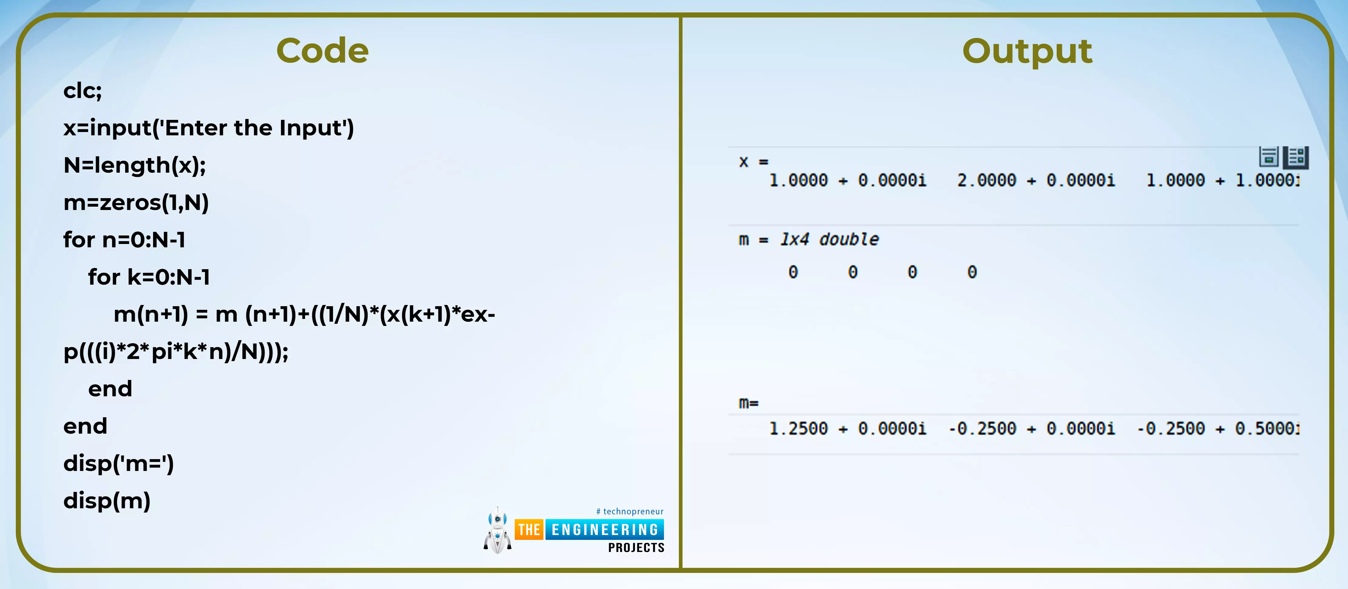
4. Why is the Discrete Fourier transform important?

5. Why is the fast Fourier transforms named so?

6. How can you implement a fast Fourier transform in MATLAB?

What is the Fourier Transform?

Just like the Laplace transform, the Fourier transform is also named so because of the name of its inventor. It is a 200 years old transform that is still in use in mathematical subjects in which there are minute calculations and the user wants to have accurate results in a simple way. The name of this transformation is taken from the French mathematician Jean-Baptiste Joseph Fourier. From 1807 to the current age, people found this transform useful, and when we talk about subjects like signals and systems, it becomes necessary to learn this because it is majorly used in the field of practical work. We define the Fourier transform as:

“The Fourier transform is a mathematical tool or model that is used to generalize the Fourier series in a simple way and is used to represent the calculator in the frequency domain.”

The definition must be clear in your mind because we have read about the transform before, but for a clear discussion, let me say that this transform is used to convert complex calculations into a simpler way by changing the domain of the values so that we may get the best results accurately in less time.

Mathematical Form of Fourier Transform

The complex Fourier series is converted into the one with the limit from minus infinity to plus infinity. The mathematical formula for this transform is given below:

At first, this formula may be confusing for you. But do not worry, when we discuss the details, you will get a clear idea. For now, keep in mind. This is also called the forward Fourier transform. We will also learn about the inverse FFT in the coming session. 

What is the Fourier Series?

You can see that we have taken the name of the Fourier series in the introduction given above. If you are new to this, let us recall.

“A Fourier series is the one in which the decomposition of periodic functions occurs and we get the sinusoidal components that have an infinite sum of sinusoidal functions.”

 It is important to introduce the Fourier series when solving the Fourier transform. Whereas a periodic function is the one that follows the formula given below:

f(t+T) = f(t)

It means that a periodic function has the same value before and after a certain period, and no change occurs after that period. 

The Story Behind the Fourier Transform

The story of Fourier's transform starts in 1807 when Jean-Baptiste Joseph Fourier found that he could represent the summation of sinusoidal functions that are sine and cosine. He worked hard on the same topic, and his work was published under the title "Analytic Theory of Heat" because he used his work to find the calculations of heat. Moreover, after this publication, scientists found that this theory can also work in other ways. It is possible to use the Fourier series of the amplitude of a sinusoidal function when the integer is used in this work. Hence, other studies were also used with the Fourier series and, as a result, many useful invasions and calculations occurred. 

Types of Fourier Transform

In computer-based applications, you will hear a lot about two types of Fourier Transforms:

1. Discrete Fourier Transform or DFT

2. Fast Fourier Transform or FFT

We will discuss both of them in detail.

Discrete Fourier Transform or DFT

We all know that discrete quantities are those with a non-continuous sequence. These are different ways to deal with signals, but when we talk about DFT, one must know that it is one of the most accurate and powerful tools to find the spectrum when dealing with finite duration signals. 

For instance, take the case in your mind, when we get the output of the LC oscillator, we get a sinusoidal wave, and we want to know the amount of noise in the output to find an accurate result, then we use the Discrete Fourier Transform. Just like digital filters, DFT is also a powerful tool to analyze the signals in the best way. 

Mathematically,

To make a clear difference between DFT and DTFT (you will learn more details soon), we have shown this equation with the variable X(k). Here, 

N =Total number of samples

j, k = variables

Pay heed to the formula and you will see that it consists of some finite numbers. Therefore, we can say that DFT is used to determine the spectrum of the sequence with a finite number of samples. 

Fast Fourier Transform

Here is another type of Fourier transform that, as the name implies, is a fast method of performing Fourier transforms. Have a look at the simplest definition of this simple Fourier transform:

“FFT is the type of Fourier transform that converts the signal into a single spectrum and, therefore, it provides the information about the frequency of that signal easily."

Let’s hear the story of the simple signal when it is fed into different procedures of FFT. 

• First of all, the signal is decomposed into a complex N time domain signal that is a complex signal. This signal has two parts:

1. Real part

2. Imaginary part

• Then different procedures occur at these parts. They are multiplied, and we get different chunks of information. 

• After all the information from the N-1 number of samples is collected, the procedure to merge all the information into a specific pattern starts. 

• Once we get the information in that particular sequence in the frequency domain, we use the calculations to get the final result. 

You might be wondering why this method is named "fast transform." Well, FFT is the form of DFT that skips some procedures, and in this way, we get a short form of the Fourier transform that is fast to perform. 

It is a fast algorithm that works on the rule of divide and conquers. It takes the signal and divides it into two smaller signals. In this way, it becomes easy to solve the signal. 

FFT in MATLAB

Code:

t=0:0.01:1;

x=sin(2*pi*15*t);

subplot(211)

plot(t,x)

xlabel('Time /The Engineering Projects.com')

ylabel('Amplitude')

FFT=fft(x,1024);

xabs=abs(FFT);

subplot (212)

plot(xabs)

ylabel('Amplitude')

Output:

The FFT Function in MATLAB

As you can guess, it is the pre-defined function to perform the Fourier Transform, and we just have to provide the parameters, and all the tasks and calculations are here in front of you in seconds. The syntax of the FFT function is given as

1. fft(x)

2. fft(x,y)

3. fft(x,y, dim)

Where

x is the equation that we want to use to perform the FFT.

y represents the number of points for the DFT.

Dim is the dimension of the Fourier transform. If you have any, you can write them here. 

In our code, we have used the second form. It is up to you which kind of syntax you want to use. The more details you provide to MATLAB, the better results you will get. 

Abs function in MATLAB

Another function that we have used in MATLAB is the abs function called the absolute function. This function is used to have the absolute values in the MATLAB codes. The result we obtain from the fft function may have real and imaginary parts or it may also have some negative values in it that are complex to deal with. For our convenience and the accuracy of the result, the abs function converts it into the absolute value that has the positive integers and we get the accuracy in our answer. 

Explaining FFT in MATLAB

While looking deeply into the code given above, we can understand the concepts of the fast Fourier transform. Here is the flow of code through which we are performing it:

• First of all, t specifies the time period at which the Fourier transform will be shown on the graph. Here, we have provided the starting point as 0 and the ending point as 1. The value between them is the period on the basis of which the shape of the wave will be shown. 

• To store the equation of the Fourier transform, we have used the variable x. This is the basic question and as we all know, there is a compulsion to write the signs of arithmetic operations and brackets all the time. 

• The result is then fed into the plot command where we specify the time on the x-axis and the value of the question that we have saved in the x variable is specified on the y-axis.

• The whole work is done by the single function of fft. You just have to input the values and you will get the result. 

• To improve the work of this transform, we are using the abs function. 

You can also use the same function without the plot and subplot commands if you do not want any graph. Take it as your homework and find what value you get when you simply put the value of x in the fft function. The results will be shown on the right side of the screen and each value can also be examined separately as we have specified in our code. 

Discrete-Time Fourier Transform

In addition to the two types, we also experience another type of mathematical tool named the Discrete Time Fourier Transform. At first, you may think it is DFT, as we have discussed before, but in reality, it is a slightly different form of Fourier Transform, and it is important to know about it so that you may clear some concepts. 

The Mathematical Form of DTFT

Once you get an idea of its application, you can understand the mathematical form of DTFT. If for a given spectrum of signals, we have the sequence named x(n) then the DFT of that particular sequence can be found with the help of this general formula given below:

Note that x(n) is in the form of time domain signals. whereas the resultant  X(ω) is in the form of a frequency domain with the complex variable ω that is omega.

There is a different notation on the same formula on the internet with different types of variables. So, do not be confused and get the core concept and apply it in your own way. 

The Difference Between DFT and DTFT

Today we have learned a lot about the Fourier transform and also seen some practical implementation of some types of Fourier transform. We have introduced the Fourier transform, learned about the type of this transform, and also saw the DTFT with the comparison of DFT. The code on the FFT was explained deeply where we had the details of its function and also saw the graph as a result. We have a lot of information about the Fourier transform, and we are going to discuss it in detail in our next session.