Types of Convolution in MATLAB

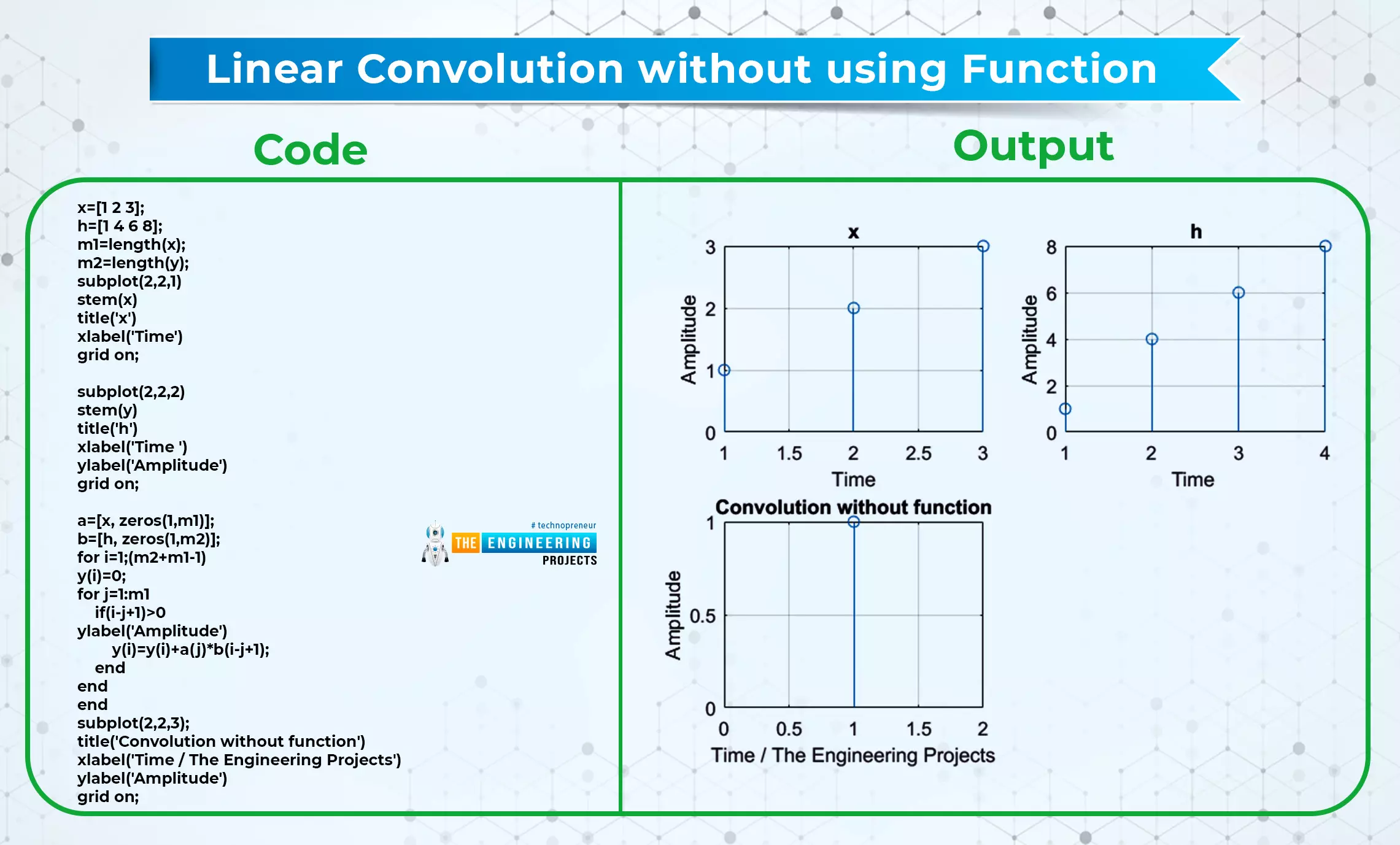
Hey pupils, Welcome to another lecture of this series on signals and systems, and this is the time to learn an interesting topic in which you are going to learn about the convolution of the signals. In the previous sessions, we have learned basic operations on the signals, and this time, you are going to know the convolution of the signals and different criteria that are related to this topic. Have a quick view of the concepts that will be clarified in this lecture:

  • What is convolution?

  • What are some basic types of convolution?

  • How can you define the properties of linear convolution?

  • How can you implement convolution in MATLAB using function and without function?

  • What is the difference between linear and circular convolution?

What is the convolution of signals?

Convolution is a mathematical operation and it is widely used in signals and systems by using a minimum of two signals at a time. The basic definition of convolution is:

The term "convolution" refers to a mathematical process combining two signals by overlapping them to produce a third signal.

It is important because it establishes a connection between the system's input signal and the impulse response of the system, which determines the system's output, which is utilized to provide a relationship within the LTI system.

Before going into details of the convolution, you must have the idea of shifting and scaling that we have discussed before in this series. Let’s recall them.

"Time shifting" refers to moving a signal forward or backward in time. The time variable in the function is multiplied by the shift or subtracted from it to do this."

Hence, convolution is an integral function that is used to measure the amount of overlap of one function when it is shifted over the other function.

The formula of Convolution

If the definition of convolution is clear to you, then you can easily understand the formula for it.

We all know that there are two types of signals and, therefore, there is a different representation of the formula of convolution in each type.

Convolution of a continuous-time system:


Where,

y(t) = convoluted result

x(t)= 1st function

h(t)= 2nd function


Convolution for a discrete-time system:


Similar to the 1st case,

y(n) = convoluted result

x(n)= 1st function

h(n)= 2nd function

The steric sign here represents convolution, and it is the most important part of this formula. Do not be confused with the symbols of t and k in continuous and discrete signals, respectively. These are the dummy variables of the result so that the input and output representation must not change.

We are not going into details of the derivation but for the clear concepts, let’s solve the example to have practice.

Types of Convolution

Basically, there are two types of convolution that are used in signal and system. These are

  1. Linear convolution

  2. Circular convolution

A brief description of each of them is given next:

Linear Convolution

This is the basic type of convolution and is defined as:

“The calculation of the output of any Linear-Time Invariant (LTI) system, given that system's input and impulse response, is done with the help of a mathematical procedure known as linear convolution.”

Till now, the properties and procedures that we have discussed were related to linear convolutions. One thing that must be kept in mind is, that the arrow on the values of x(t) and h(t) indicates the zero position of the function. If this arrow is not specified, then by default, the first value is the zero value.

Procedure for Linear Convolution of Signals

You will find different formulas to have the convolution of signals, but here, we are providing you with the basic and easiest way to solve the convolution without any confusion. Just follow these simple steps to get the convolution.

  1. Replace T with t

  2. Time reversal in h(t)= h(-t)

  3. Time shifting in h(t)= h(t-t)

  4. Multiplication of h(t-t) with x(t)

  5. Integration of the result by taking the limits from minus infinity to infinity

Keep in mind, in all the steps, the value of x(t) remains the same and just t is replaced by t i.e, time reversal and time shifting do not apply to x(t) while you are using the convolution.

Circular Convolution

The other type that I found more interesting in the convolution of signals is circular convolution. This type can be performed using two different methods, and by observing the procedure of each type, you will understand why this type is called “Circular” convolution. The total number of samples in circular convolution is equal to the maximum number of values in x(t) or h(t). Have a look at both of these:

  1. Concentric circular convolution

  2. Matrix circular convolution

We are going to discuss both of them in the next section.

Concentric circular convolution

Here, you need a circle for each signal or function. In this way, you will have two circles. Follow the steps from the beginning as mentioned below:

  • Draw a big circle on the page and write the values of x(t) on it at regular intervals.

  • Draw a relatively small circle inside the first one and write all the values of h(t) on it at the same regular intervals.

  • Multiply the respective values of both the circles and at the end, add them all. You will get a number.

  • Now, draw the same circle once again but this time, you have to move the internal circle (the one with h(t) values) one place anti-clockwise and then repeat the above procedure till you get all the values.

Matrix circular convolution

The matrix multiplication, as the name implies, consists of two matrices having the values of x(t) and h(t) respectively. The simple steps involved in this method are:

  • One of the given sequences is repeated, one sample at a time, to produce an N X N matrix.

  • The other sequence is shown as a column matrix.

  • The outcome of circular convolution is obtained by multiplying two matrices.

Convolution Procedure in MATLAB

Here comes the action. You have seen that there were different ways of convolution, and honestly speaking, these procedures are long yet easy. MATLAB has built-in functions for convolution so that you may get the answer to long and time-taking calculations in just a bit. You just have to simply input the values, and tell MATLAB that you want to do the convolution of this signal. Let’s implement all the discussions in MATLAB and get the instant and authentic result of convolution there.

Step for Linear Convolution in MATLAB

  • Fire up your MATLAB software.

  • Go to live editor or command window to write the code.

  • Click the “Run” button.

  • Save program.

Linear Convolution using Function

There is a built-in function in MATLAB that is super easy to use, and you do not have to go deep into the procedure. You just have to simply provide the input signals and use the convolution function. If x and h are two signals that have the values, then using this function, you can easily convolute them as

conv(x,h)

At the end, you just have to simply put this value in the y variable so that you can plot or stem it easily. Here is the code and output.


Code

Output

x=[1 2 3];

h=[1 4 6 8];

y=conv(x,h);

stem(y)

title('Convolution using function')

xlabel('Time / The Engineering Projects')

ylabel('Amplitude')

grid on;


Linear Convolution without using Function

It may come into your exam that you are required to perform the linear convolution but without the help of function. Usually, it happens when the instructor wants to check the knowledge and concept of the student. So here is a simple program for this.


Code

Output

x=[1 2 3];

h=[1 4 6 8];

m1=length(x);

m2=length(y);

subplot(2,2,1)

stem(x)

title('x')

xlabel('Time')

grid on;


subplot(2,2,2)

stem(y)

title('h')

xlabel('Time ')

ylabel('Amplitude')

grid on;


a=[x, zeros(1,m1)];

b=[h, zeros(1,m2)];

for i=1;(m2+m1-1)

y(i)=0;

for j=1:m1

if(i-j+1)>0

ylabel('Amplitude')

y(i)=y(i)+a(j)*b(i-j+1);

end

end

end

subplot(2,2,3);

title('Convolution without function')

xlabel('Time / The Engineering Projects')

ylabel('Amplitude')

grid on;


Circular Convolution in MATLAB

Circular convolution can also be done with the help of function and without it as well. Of course, it is easier to use the function, but in some cases, if you do not want to use the function, it is also possible to do it without the help of the function. The difference between the formulas is, that the circular convolution involves the third parameter as well. This value is obtained when the total number of values of signals is compared and we get the maximum value. For a practice point of view and to clear up the concepts about the topic, we are also using it without any function.


Code

Output

x=[2 2]

h=[1 1 1]

l1=length(x)

l2=length(h)

N=max(l1,l2)

a=cconv(x,h,N)

subplot(2,1,1)

stem(a)

title('Circular Convolution with Function')

xlabel('Time / The Engineering Projects')

ylabel('Amplitude')

grid on;

x=[x zeros(1,N-l1)]

h=[h zeros(1,N-l2)]

y=zeros(1,N)

for n=1:N

for m=1:N

j=mod(n-m,N)

j=j+1

y=y+x(m)*h(j)

end

end

subplot(2,1,2)

stem(y);

title('Circular Convolution Without Function')

xlabel('Time / The Engineering Projects')

ylabel('Amplitude')

grid on;


Length Function

Similar to some other functions, length is also a function of MATLAB that stores the output of the number of values that are fed into this function. Let's suppose if the number of elements on the x-axis in a signal is ten and we feed the signal into this function, then it will provide us with the length of 10. It may seem simple, but in complex signals where a hundred or thousand values in a signal are used, this function proves very helpful.

The Max function in MATLAB

Have you observed a function “Max” in the code? It is a built-in function of MATLAB that compares the entries and provides you with the entry (signal in our case) with the maximum number of values. Usually, the answer is then fed into a variable so that we can use the result of this max function anywhere without any difficulty.

For your information, we must share that there is another function named "min", and as you can guess, it does the opposite work. Two or more values are given to this function as well and it compares and then provides the minimum value between these two. It may seem a small task but if used correctly, these functions give us control of many useful things by using them in our program.

Difference Between Linear Convolution and Circular Convolution


Linear Convolution

Circular Convolution

Complexity

Less Complex

More Complex

Shifting

Linear Shifting

Circular Shifting

Numbers of samples

N1+N2-1


Max(N1, N2)


Types

Not common types

Concentric circular convolution, Matrix circular convolution

Formula in MATLAB

conv(a,b)

cconv(a,b)


Conclusion

Convolution is an important topic in signals and systems as it is used to overlap the two signals on each other in such a way that a third signal is obtained that is different from the first two. We have read some important properties of linear convolution and also seen the performance of each type with and without the function in MATLAB. The purpose of providing the program of convolution without function is to clearly describe the concept and the method of convolution. If you have any type of question regarding the topic, you can contact us.

Classification of Systems

Hello Pupils, We are learning about signals and systems, and till now we have learned some basic information regarding signals, but we know a little about systems till now. We have learned about the system in our previous lectures. To have a clear concept, we have arranged this tutorial in which we are studying the systems and their classification. Have a quick glance at today’s topics:

  1. What is a system?

  2. What are the various types of systems?

  3. What is the principle of homogeneity?

  4. What is the principle of superposition?

  5. How can we compare each type while keeping their differences in mind?

To keep things simple, we’ll also have examples of some of these signals. Yet, the first thing that we are going to do is to revise the basic definition of the system so that we may move forward.

What is a System in Signal and Systems?

A system is a closed connection between the input signal and the output. All the procedures and techniques required to convert the input into output are called the system, and if we talk critically, then the basic definition of a system is:

“A system is a collection of components that, when interconnected, provide a signal that is proportional to the signal that was fed into the system.”

To understand, keep in mind, that the system has the input where the data is fed, then different procedures take palace on that data, and as a result of this procedure, we get the output from the system. 

Classification of Systems

As with signals, systems also have some types, and these types are clearly classified for convenience. We will go through some basic types and will try to have a clear concept through discussion and examples. 


Linear and Non-Linear System

There are different ways to define the linearity of the system, but the easiest one is, that a system is called linear only if it follows:

  1. Principles of homogeneity

  2. Principle of Superposition


We’ll define both of them one after the other in detail.

Principles of Homogeneity

According to the concept of homogeneity, a system that produces an output y(t) for an input x(t) must also provide an output ay(t) for an input ax. This is the condition that must be met for the system to be considered homogeneous (t).

Principle of Superposition

According to the concept of superposition:

“A system that produces an output of y1(t) for the input of x1(t) and output of y2(t) for the input of x2(t) must create an output of [y1(t) + y2(t)] for the input of [x1(t) + x2(t)]. Similarly, [y1(t) + y2(t)] for the input of [x1(t)], and implies any number of different signals in the system. "

Well, is it confusing? Do not worry because we are discussing it in simple words. Consider the case when the system has more than one signal in it. If we provide it with 3 signals (let’s say) at the input, then the output contains the collective effect of all the signals that we were expecting from each and every signal by adding them. 

It may make no sense at the time because every person, after using their commonsense, can make this decision on their own, but keep in mind that these types of principles are highly effective in solving the complex problem of calculations. 

As a result, when we plot the graph of a linear system, we find a simple and clear graph that is usually straight in line. It is the reason behind calling them “linear”. It is usually easy to deal with the linear system as compared to the other type that is non-linear. The reason behind this will be discussed in just a bit. Before that, have a look at the diagram given below:


Non-Linear System


On the other hand, if the system does not obey the principles of superposition and homogeneity, then it is called non-linear. It is not possible to develop a general differential equation of finite order that can be utilized as the mathematical model for all systems when dealing with nonlinear systems; this is because such an equation would be impossible to solve. This is due to the fact that there are numerous distinct paths via which nonlinearities might emerge, and these paths cannot all be mathematically expressed using the same form. In addition to this, it is essential to keep in mind that the concept of superposition cannot be applied to nonlinear systems.


Continuous-Time System

Let’s talk about a very simple and obvious type of system. A system is called a continuous-time signal if the input given to it, and the output obtained from it, both are continuous-time signals. The operations done on the input do not change the form of the input signals and hence the output is not affected in its shape and type. 

Example

A simple example of a continuous-time signal is an amplifier in which the input is analog in the form of voice. Different procedures occur inside the system (amplifier), and from the output, an amplified voice (analog signal) is obtained from it. 

Discrete-Time System 

As you are expecting, a discrete-time system is one in which the input given to the system and the output obtained from the system, after different procedures, are in the form of discrete-time signals. If in any case, the system changes the signal from discrete to continuous, then it will not be a discrete-time system. 

Example

Micro-processor is an example of a discrete-time signal because all the processes that occur in the micro-processor are based on just two numbers that are zero and one and the output, after different operations, remains in the same format. 


Invertible System

In some cases, the same results can be obtained from the output of the system that was fed into its input signal, and such systems are termed invertible systems, as the name implies. We define them as:


“A system is said to be an invertible system if it is designed in such a way that the input, that is fed into the system goes through some changes and these changes can be converted into the original signal again by using the different procedure and the input is equal to the output.”


Practically, an invertible system is obtained by using a system in which, in addition to the simple system, an inverter or any other device, that has the opposite mechanism is cascaded to obtain the same input and output.

Moreover, another way to do so is to have more than one input and choose them in such a way that different inputs cancel out the result of each other and we get the same resultant output as the inputs. 

Non-invertible System 

The system in which the input and output are not equal is called non-insertable. We define them as:

“A system is said to be non-invertible if the effect of the system, exerted on the input signal, can not be inverted. No matter which procedure you are following inside the system, you will get different inputs and outputs. “

Time-Variant Systems

Time-Variant systems are those whose output depends upon time. We know that every signal has time on the x-axis but keep in mind, in a time-variant system, a signal depends upon the change in time. 

Example

The example given below represents the case of a time-variant system:


y(n)= x(-n)

Time-invariant System

The system is said to be time-invariant if the output of the system does not depend upon the time of the system.

Example

Consider an example in which the output is called y(t) and the input is represented as x(t). Then the equation given below presents the time-invariant system:

y(t)=x(t)+x(t-1)

Static System

Here is another type of system. We all know that static means motionless or unchanging condition. A static system is one that depends upon a particular result at a particular time and it does not have any relationship with the previous or future results. 

“A static system is the one that depends upon the present situation only and does not have any mechanism to store the past or future value because it does not need to store these values”.


Example

𝑐(𝑡) = 𝑟(𝑡)

𝑐(𝑡) = 2𝑟2(𝑡)

In these examples, the whole system depends upon the time at a particular instant, and it does not have any concern with the previous or upcoming value. This will be more clear when you look at the example of the dynamic signal in just a bit. 

Dynamic System

Dynamic means anything that is not stationary. In the case of signals, the dynamic signals are the ones that depend upon the present, past, and future values of the signals. Have a look at the definition:


“A dynamic system is one that can not be achieved by using the present values of the signals only; instead, they also depend upon the future and past values, and therefore, they require memory to store the previous results." 


Example

A simple example of a dynamic system is the capacitive system. The capacitor is used to store the charges, so they are also used to store the memory in computers, and the discharging process depends on the number of charges stored an instant before. Therefore, we consider it a dynamic system. More examples are inductive circuits, delay circuits, accumulators, etc. 

Casual System

Have a deep look at these signals. These are the ones that totally depend upon the present and past values of the signal but do not have any concern with the future values. 

Keep in mind, that these are not the same as the static or dynamic system, but are slightly different from them.

Non-casual System

In non-casual systems, the system depends upon the past, present, and future values, and if any of them is missing, the system is not able to work properly.


Summary

We are going to end by discussing the summary of the whole article. We have ready many types of signals and, similarly, systems also have some classification. Most types of systems have an opposite type as well and for convenience, we have discussed them one after the other so that you may compare them and have a clear idea about them.  We have discussed some common types of systems and the key points of each type are given below.


System

Features

Linear system

  • Follows the principles of homogeneity and superposition.

  • Simple 

Non-linear systems

  • Do not follow the principles of homogeneity and superposition.

  • Complex


Continuous system

  • Depends upon continuous values.

  • Input and output are continuous signals.

  • Amplifier is an example.


Discrete system

  • Depends upon discrete values.

  • Input and output are discrete signals.

  • Microprocessor is an example.


Invertible system

  • Planned in such a way to invert the signal at the output.

  • Input is equal to output in all ways.

Non-invertible system

  • Mechanism is present in such a way that the input can not be inverted. 

  • Input is never equal to output.

Time variant system

  • The output depends upon time and varies from time to time.

Time-invariant system

  • The output does not depend upon time.

Static System

  • Memory-less system.

  • It does not have any concern with past or future value. 


Dynamic System

  • Memory is necessary for this system.

  • It has a strong concern with past or future value. 

  • Example: capacitive systems.

Casual system

  • The output depends on the past and present values only.

Non-casual system

  • The output depends upon the past, present, and future values.

Conclusion

There are numerous types of systems in which the type of input and the type of output are strongly examined to know the particular type of system. For the best understanding, keep the difference between each of them in mind. There may be other types as well yet for this course, these types are more than enough. You should go through them and find the examples of each of them by summing up your concepts and common sense. You must keep in mind, that a system can be of more than one type at a time. We will go through the next topic in the next step.

Basic Operations on Signals in MATLAB

Hey peeps welcome to The Engineering Projects. This is the third lecture of this series, and till now, we have discussed the introduction to the signal and system, and in the previous lecture, we learned about the classification of signals and the difference between some of them. 

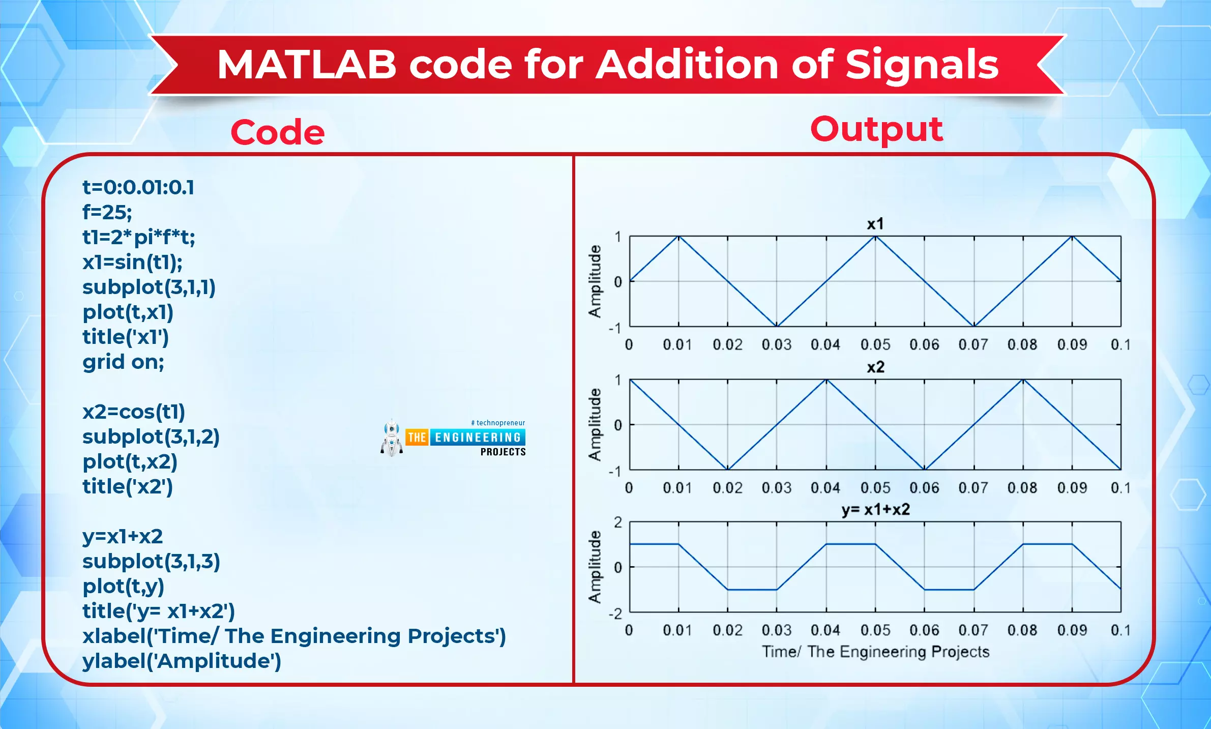
In the present day, you are going to learn the basic operations of signals, and it is amazing to note how you can play with these signals. The best thing about this series is that you are going to see every step with the help of MATLAB. Let’s have a quick glance at today’s topic, and after that, we will go through a detailed explanation.


  1. Addition of Two Signals

  2. Subtraction of Two Signals

  3. Multiplication of Two Signals

  4. Time Scaling (Compression and Expansion)

  5. Time Shifting (Addition and subtraction)

  6. Reversal of Signal

Moreover, you will also learn some practical applications of some of these operations. All these operations are explained with the help of MATLAB code, and for simplicity, the codes are kept basic so that you may learn more about the concepts. 

Basic Concept

Keep in mind that a signal has some parameters on the basis of which its graphical representation gets a face. These parameters are

  1. Time

  2. Amplitude

In all the operations, we will deal with these two parameters and change their values in different ways. Recall in mind that the greater the amplitude, the longer a signal goes on the y-axis and more time means that we’ll get wider loops of the signals. Time is an independent quantity and it is always kept on the x=axis no matter what type of signals are you dealing with. In each signal, when working on MATLAB, you will put the time in the first place from the left when using the Stem or Plot function.


Operations on the Signals

Addition of Signals

We are starting with the easiest operation of the wave. The addition of the signal is the process in which the amplitude of two signals is added and as a result, the signal obtain has the combination amplitude of both of these. The simplest example of this operation is:

x1=sin(2πt)

x2=cos(2πt)

y=x1+x2

The resultant Y has the value of the addition of both these signals. Have a look at the same result on MATLAB for the best graphical representation.

MATLAB code for Addition of Signals


Code

Output

t=0:0.01:0.1

f=25;

t1=2*pi*f*t;

x1=sin(t1);

subplot(3,1,1)

plot(t,x1)

title('x1')

grid on;


x2=cos(t1)

subplot(3,1,2)

plot(t,x2)

title('x2')


y=x1+x2

subplot(3,1,3)

plot(t,y)

title('y= x1+x2')

xlabel('Time/ The Engineering Projects')

ylabel('Amplitude')


Keep in mind, this is not the amplitude at which the operation of addition takes place but the values of the amplitude are summed up and MATLAB store these values and show you another wave of this. You can match the values of the result from the workspace window or simply have a look at the wave. Let’s start from the initial point:

y=x1+x2

At point 0


1=0+1

At point 0.01


1=1+0

At point 0.02


-1=0+(-1)

And so on.

Subtraction of Signals

Subtraction is also possible in the signals, just like the addition operation. Subtraction between the two signals takes place when the value of the second signal (the one that is written after the subtraction sign) is subtracted from the first signal. 

In MATLAB, for simplicity, we are using the same code with the value of subtraction between x1 and x2. 

MATLAB Code for Subtraction of Signals


Code

Output

t=0:0.01:0.1

f=25;

t1=2*pi*f*t;

x1=sin(t1);

subplot(3,1,1)

plot(t,x1)

title('x1')

ylabel('Amplitude')

grid on;


x2=cos(t1)

subplot(3,1,2)

plot(t,x2)

title('x2')

ylabel('Amplitude')

grid on;


y=x1-x2 % Here the subtraction takes place

subplot(3,1,3)

plot(t,y)

title('y= x1-x2')

xlabel('Time/ The Engineering Projects')

ylabel('Amplitude')

grid on;

Here, you can check the output that is almost the inversion of the addition result because of the inverted sign, and hence the output is justified easily. 

Multiplication of Signals

Okay, you must think that this will be the same as the previous two concepts, but no. There is something different from the previous one, but before exploring that, let’s just define the multiplication of the signals:

“The multiplication of two signals is obtained when the values of the amplitude of two signals are multiplied and the resultant signal has the multiplied amplitude.” 


Have a look at the MATLAB code.

MATLAB code for Multiplication of Signals


Code

Output

t=0:0.01:0.1

f=25;

t1=2*pi*f*t;

x1=sin(t1);

subplot(3,1,1)

stem(t,x1)

title('x1')

ylabel('Amplitude')

grid on;


x2=cos(t1)

subplot(3,1,2)

stem(t,x2)

title('x2')

ylabel('Amplitude')

grid on;


y=x1.*x2 % Here the multiplication takes place

subplot(3,1,3)

stem(t,y)

title('y= x1*x2')

xlabel('Time/ The Engineering Projects')

ylabel('Amplitude')

grid on;


When we use the simple steric sign (star/multiplication), then you will not get the output and instead a blank output will appear on the screen. It is because, without a dot, MATLAB performs the operation of an array operation, but for the multiplication of a single element with other single elements, we need the matrix type of multiplication.

Time Scaling of Signals

If you are new to signals and systems, this is something different that you will learn for the first time. At first, you may think that it is a simple multiplication of signals, but soon you will realize that only one signal is used in this operation, the opposite to the case that we have discussed earlier. Have a look at the definition of this operation:

“The term time scaling refers to the process of multiplying a constant by a signal's time axis. This technique is also known as time scaling of the signal."


Depending on the magnitude of the constant or scaling factor, the time scale of a signal has two possibilities:

  1. Compress

  2. Expansion

These two processes occur depending on the amount of time it takes to complete the signal. 

Compression in Time-Scaling

Compression of the signal occurs when the constant number, multiplied by the signal is greater than zero and as a result, a signal is obtained that has a less wide form than the parent signal. It is because the time axis has more values in the resultant signal.  

Expansion in Time-Scaling

You can say it is the opposite phenomenon of the compression of the signal. In this process, the constant number that is multiplied by the signal is less than zero, and therefore, the gained signal has a wider form. 

When data is to be brought in at a certain rate and taken out at a different rate, the time scaling operation of signals is a highly helpful tool to have. It will be more clear when you will observe this example:

MATLAB code for Time Scaling of Signal


Code

Output

t=0:0.01:8*pi

x=sin(t);

subplot(3,1,1)

plot(t,x)

title('Simple Signal')

xlabel('Time')

ylabel('Amplitude')

grid on;


y=sin(t/2)

subplot(3,1,2)

plot(t,y)

title('Expanded Signal')

xlabel('Time')

ylabel('Amplitude')

grid on;


z=sin(t*2) 

subplot(3,1,3)

plot(t,z)

title('Compressed Signal')

xlabel('Time/ The Engineering Projects')

ylabel('Amplitude')

grid on;


Applications in the Real World

Changing the rate at which the signal is sampled is the primary focus of the time scaling technique that we employ. Altering the frequency at which a signal is sampled is one technique that is used in the field of voice processing. A system that is based on a time-scaling algorithm that was built to read text to people who are visually impaired is a specific example of this.


Time Shifting of Signals

This is another operation on the signal in which the x-axis or time axis changes. Instead of changing the width of the signal, we are shifting the wave to a different location on the x-axis. 


“The process of moving a signal forward or backward in time is what the term "time shifting" refers to. To do this, either an additional amount of the shift or subtraction from it is applied to the time variable in the function.”


It is interesting that you are moving the whole signal on the time axis. It has two processes:

Addition in Time Shifting

This process is used to move the whole signal to the right side of the time axis. The whole signal moves towards the right side and the amplitude does not change. 

Subtraction in Time Shifting

As you can guess, by subtracting the value on the time axis, you can simply move your signals to the left side of the x-axis no matter where they are at the start. 


MATLAB code for Time Shifting of Signal


Code

Output

t=0:10;

x=[0 1 2 1 0 1 2 0 1 2 1 ];

subplot(3,1,1)

plot(t,x)

title('Simple Signal')

xlabel('Time')

ylabel('Amplitude')

grid on;

axis([-2 8 0 4]);

subplot(3,1,2)

plot(t+2,x)

title('Shifting by addition')

xlabel('Time')

ylabel('Amplitude')

grid on;

axis([-2 8 0 4]);

subplot(3,1,3)

plot(t-2,x)

title('Shifting by Subtraction')

xlabel('Time/ The Engineering Projects')

ylabel('Amplitude')

grid on;

axis([-2 8 0 4]);


In this example, we have just added and subtracted the values of the time axis and the whole signal is shifted from one place to another. For convenience, we have just added and subtracted two numbers. You have to focus on the values of the x-axis. 

Applications in the Real World

A significant number of signal-processing applications make use of an operation known as time-shifting, which is an essential procedure. For the purpose of performing autocorrelation, for instance, a version of the signal that has been time-delayed is utilized.


Time Reversal in Signals

When one is first learning about time scaling, one of the most natural questions to ask is, "What happens when the time variable is multiplied by a negative number?" Time travel is the solution to this conundrum. This procedure inverts the time axis, often known as flipping the signal over so that it reads along the y-axis.

“ The process of flipping the whole signal by using the flipping function or by multiplying the whole signal with a negative number is called reversal of the signal because each and every value of signals is reversed”.


This technique is useful in many cases, and the best thing is, that you do not have to change your code much. Just 1 step and you are good to go.


Code

Output

t=0:10;

x=[0 1 2 3 4 -5 -6 -7 -8 -9 -10];

subplot(3,1,1)

stem(t,x)

title('Simple Signal')

xlabel('Time')

ylabel('Amplitude')

grid on;

y=fliplr(x);

subplot(3,1,3)

stem(t,y)

title('Shifting by addition')

xlabel('Time')

ylabel('Amplitude')

grid on;


Conclusion

There are certain operations on the signals that are too easy to perform but have the ability to change the working of the entire signal. These operations work as the backbone of the signal and system, and once you have command of this, you can work more deeply with the signals. You may also see some other operations in the upcoming tutorial, but for now, you must practice these basic operations and try to make your own signals and play with them. It is an interesting task that must be done on the same day as you learn the basic definition of these signals.

Syed Zain Nasir

I am Syed Zain Nasir, the founder of <a href=https://www.TheEngineeringProjects.com/>The Engineering Projects</a> (TEP). I am a programmer since 2009 before that I just search things, make small projects and now I am sharing my knowledge through this platform.I also work as a freelancer and did many projects related to programming and electrical circuitry. <a href=https://plus.google.com/+SyedZainNasir/>My Google Profile+</a>

Share
Published by
Syed Zain Nasir