Subroutine in Ladder Logic Programming

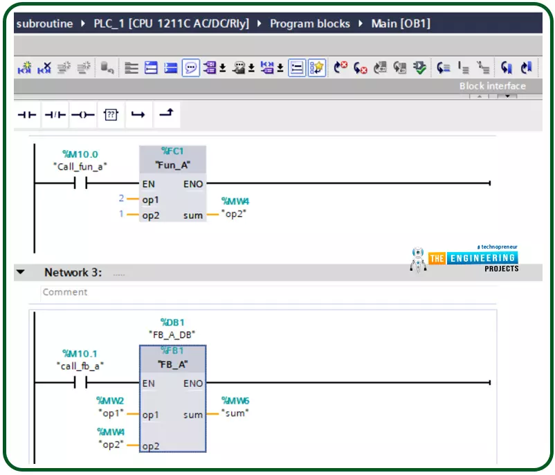
Hello friends, after completing that basic part of ladder logic programming, let us today go through one topic which is not essential to know to complete a PLC ladder program but it is important t have our code readable program and reusable pieces of code. That could happen by using what so-called a subroutine. So what is a subroutine?

Well, it is a piece of code that includes a few rungs to perform specific tasks. that piece of code can be reused numerous times through the program when we need to call it for performing that task. That subroutine enables us to structure our code like building blocks so that the program will be readable very easy and also reusable later in other projects. The idea of dividing the program into routines to apply the divide and conquer technique is very crucial to ease the coding of your program especially when it comes to the large-scale program which is the common cause in the best industry practice.

Each routine achieves one specific task and they are integrated to accomplish the whole mission. By programming in that way, the code is more readable and reusable meaning that one routine could be called many times instead of keeping repeating the lines of code or ladder rungs everywhere we need it. In this tutorial, we are going to be very familiar with subroutine-based programming including different ways to call a subroutine and the instructions that are used for handling subroutines. And yes we are going to practice examples that program that subroutines in ladder logic so let's get started.

Types of routines 

Routines can be classified into two main types: the calling routines that call subroutines. And routines that are being called. Figure 1 shows the very typical scenario of calling one subroutine. It shows the scenario when the calling routine reaches the calling instruction when the subroutine is being called with the value of the parameter passed by the calling routine and then the subroutine has a return instruction to take the execution to the following instruction of the calling instruction.  So you can imagine the calling instruction is in the calling routine which is mostly the main program and the called subroutine is responsible to return the control or the execution point to the instruction next to the calling instruction.

Passing parameters 

There are two main ways for passing parameters between the calling routine and the subroutine that is being called. The two ways are calling by value and calling by reference. In the calling by value method, the calling routine passes a copy of the original parameters so the called subroutine works on a copy. Therefore, there are no changes could happen to the original parameters in the calling routine. In contrast, in the second method which is called call by reference, the parameters are shareable between the calling routine and the subroutine that is being called. So, changes happened to the parameters but the called subroutine reflected on the original ones. Figure 2 depicts a case scenario of the two types of passing parameters. In that very example, the main routine calls subroutine “Call_Val” to apply an increment of operand “Op1” passing the parameter Op1 using the method “calling by value” while it calls “Call_ref” to do the same process but in that case, it passes parameter Op1 by using the method of “calling by reference”. As you can see, in the case it uses the “calling by value” method, it does not change the value of parameter Op1 because it uses a copy of the parameter and increments that copy not the original parameters. On the other hand, when it has used the other method, “calling by reference”, to increment the same parameter Op1, it does change the original operand because it uses a reference that points to the original parameter address. In another word, calling a subroutine based on a call by value works on a copy of the parameters and does not change the original variables while calling by reference works on the originally passed parameters so it does change the parameters. The advantage of calling by reference is saving the memory as it does not need an instance of the variables or a separate data block. On the other hand, calling by value needs to have a separate data block to include that copy of passing parameters. However, it can be called many times with a separate copy without any conflicts.

Program sequence:

Figure 3 shows the program sequence when using multilevel branching using subroutines. For example, the main module keeps carrying out the network net1, and net2, and it calls the subroutine “Sub x” in-network net3. Then subroutine “sub x ” starts executing from network net1 to net3 at which, it calls subroutine “Sub y”. Then subroutine “Sub y” carries out starting from the network “net 1”, and network “net 2” calls subroutine “Sub a”. You can notice subroutine “Sub a” returns to the calling routine “Sub y” which returns to subroutine to its calling routine “Sub x” which returns to its calling routine which is the main routine. So, you can notice how many levels of subroutine calls? Yes, they are a lot. But, it is recommended to be as much as needed for two reasons. First, many branching causes some headaches in processing in terms of memory and time. Memory is represented in the data block that is needed for each subroutine every single branching or subroutine calling and time is represented in extra instructions of calling and returning and stacking data related to the called routine and the returning addresses.

Subroutine instructions

There are two main instructions used for calling a subroutine and returning to the calling routine. Figure 4 shows the network rung that calls a subroutine called “Auto Mode”. It is going to call the subroutine at any time when the “System OK” memory contact MB180 is true. So I hope you can feel now how your program is more organized and readable when you go through the main program and easily can catch what the program does by reading the names of the called subroutines. Exactly, having a meaningful name for subroutines is very important to give the advantage of the readability of your program. So, my friends please make sure you chose a purposeful name for your subroutines.

Also fig. 5 shows the network rung that represents the returning command to the calling routine. It shows when the alarm is true represented by memory contact MB32 and pump status “Stop Pump” represented by memory bit64, the return command will be enabled for returning the execution point to the network just next to the calling network in the calling program. For example, if the calling network is at rung number 3, then the return command in the subroutine will return the execution at rung number 4 in the calling routine.  By the way, in most cases of ladder logic programming, you might not find a return instruction because it is inherently performed by completing the called subroutine but we just include it here as in fig. 5 to show up how the process of calling a subroutine and returning to the calling routine.

Figure 6 depicts the whole image of the scenario of calling one subroutine. In rung 3, a subroutine called “Auto mode” is being called by having the memory contact MB18 true. Then after that subroutine, “Auto mode” is completed it returns to the calling routine at the next rung to the calling rung which is in this case example rung number 4.  As we stated earlier, you can notice that there are now returning instructions but automatically, the called subroutine returns to the calling routine at the instruction just next to the calling instruction.

Practicing Subroutine in ladder logic

My friends, let us go to our lab as usual and do some hands-on practicing subroutine using the simulator. But before going further in practice subroutine we want to elaborate on the different types of subroutines in Siemens programming. Table 1 compares the subroutine implementation based on function and function block. It shows that subroutine can be implemented by either function FC or function block FB. And both ways can use input, output, and in-out parameters. 

FC does not use static data or data block (DB) while FB uses DB and passing parameters by making an instance of the variables which is calling by value. FC passes the parameter by pointing to the address of the variable which calling by reference technique.   

Table 1: Comparison between FC and FB subroutine in Siemens

Characteristic

FC

FB

Can be used as a subroutine

Yes

Yes

Can use parameters for Inputs, Outputs, and Input

Yes

Yes

Can use temporary variables

Yes

Yes

Can use static variables (with remanence)

No

Yes

Need an auxiliary (instance) DB for each call

No

Yes

Parameters are passed as the address for internal use

Yes

No

Parameters are copied to/from a DB (instance) for internal use

No

Yes

Can call internally a FB or FC

Yes

Yes

Can be called for a FB or FC

Yes

Yes

Can call a FB as multi-instance

No

Yes

Can be called without filling all parameters

No

Yes

Subroutine in ladder logic programming 

Again, there are two ways of calling a subroutine in Siemens ladder programming as shown in fig. 7. We have developed a sample ladder program that calls a simple subroutine to add two input operands. In the first rung, it uses function “FC1” called “fun_A” and in the second rung, it utilizes a function block FB1 called “FB_A” as you can notice function block uses a data block instance for passing a copy of the operands while function FC does not use a data block and uses the address of the input and output parameters.

Figure 8 shows the function block FB_A. the function block has two input operands which are “op1” and ‘’op2” and one output operand which is “sum”.

Because the function block passes parameters as copies or instances, fig. 9 shows the related data block DB1 which contains the parameters of the function block. It is composed of many structures for holding input, output, input, and static data as well.

On the other hand, the function uses the addresses of the parameters. Therefore, it does not need a data block as shown in fig. 10. It uses many structures to pass input, output, input, temporary, and constant data types.

Simulation work

Now let’s check the work with the simulator. Figure 11 shows the results of simulating the calling subroutine based on function FC_A that adds two static operands showing the calling path from the main organization block to the function.

On the other hand, calling a subroutine based on a function block uses an instance of parameters in a data block as shown in fig. 12. This means another instance of data is used every time we called that subroutine while using the function it is referencing the same variables at the same addresses. 

What’s next

Thank you guys for following me up to this very point of our tutorial and being very confident by knowing the subroutine you now are all set to write an organized program and readable and reusable piece of code using ladder logic programming. the next time we are going to talk about one of the most important topics in PLC programming which is master reset control showing what is it about and its importance for PLC and control project and for sure will practice with our simulator lab. So be ready and let’s meet in the next tutorial to enjoy learning and practice the PLC ladder programming series.

Master Reset Control in Ladder Logic Programming

Introduction 

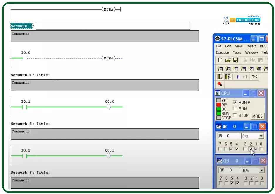
Hello friends, I hope you are doing very well. Today we are going to learn and practice the master control reset (MCR)! So what is that MCR? Well! This is a tool you might use to control a group of devices with one push button for performing fast emergency responses with one click for a group of devices in one zone. In another word, you divide the program into zones and put this zone between a master control to control their operation as one unit by one contact. This technique is useful for applying emergence stops and also protecting some equipment by applying a safety restriction to not operate when that condition is in effect. 

The concept of the master control reset (MCR)

Figure 1 shows the master control relay in a ladder logic showing a couple of rungs between the master control and master control reset to be controlled as one zone by master control. for example, input 1 enables the master control relay M100 which is the only way to relay the hotline of power to rungs 2 and 3 as shown in the figure. When input 1 is on, the master control relay is energized. Therefore, input 2 and input 3 can energize output 1 and output 2 respectively. But, if input 1 is off, the master control relay is off. Therefore, rungs 2 and 3 are disconnected from the power. Therefore, even if input 2 and input 3 are on, outputs 1 and 2 will not energize because of a missing connection to power via master control relay M100. To sum up, there is a zone that contains a couple of rungs, these rungs are not enabled without master control enabled. Also, fig. 1 shows the structure of the master control and master control reset to have one rung to enable the master control relay and one rung at the end to represent the master control reset and declare the end of the zone that is under master control. and the code or rungs that are located between the master control and the master control reset is the zone that we need to control its running based on master control. So, if the master control is not true, the code in that zone between the master control and the master control reset will be bypassed and the next instruction after the master control reset instruction will be executed. 

The concept looks very simple but it is crucial for safety and control techniques. Also, many master control and zones can have in our program as shown in fig. 2. It shows more than one zone and each one is controlled by its master control.

So we want to go further in demonstrating the master control reset by a practical example from real life. Figure 3 shows a practical example of real-life in the industry of which automatic bottle filling process. So what does master control have to do with such a process? Will! That is a good question because it tells me you understand master control reset and are with me on the same page. So, as you can see, there is the start and stop pushbuttons and we need to use master control to control starting and stopping the whole process regardless of the status of individual inputs and sensors. by having such control, we can stop the process in any emergency case or for doing maintenance. The sequence of the process is to start moving the conveyor by hitting the start push button. The conveyor keeps running until the proximity sensor comes ON. At that time, the valve will open for 5 seconds and then the conveyor continue moving again after 5 seconds and continue for 3 bottles repeating the same process. But if there is an emergency happens, there should be a way to stop the process including moving the conveyor, and opening the valve even if all conditions to do are met. Well done! You are correct, master control and master control reset should bracket the process to be enabled and disabled when that emergency comes to happen.

Master control in ladder logic

Master control and master control reset are the same concepts. However, a few differences you can notice in ladder logic from one plc brand to another. For example, Fig. 4 shows the ladder logic code of a master control reset in Mitsubishi PLC. You can notice the same concept has been applied. A zone of a couple of rungs is surrounded by master control and master control reset instructions based on master control relay M100. Input 1, X400 enables the master control relay M100. And rungs 2 and 3 are included in the zone under master control.

On the other hand, master control and master control reset look a little bit different in Allen-Bradley as shown in fig.5. However, you can notice the same concept is applied by having the zone that includes a couple of rungs between the master control relay and master control reset for enabling or disabling that zone based on the logic and situation.

Also, Siemens shows a few differences in ladder logic of master control as shown in Fig.6. however, the same concept is thereby enclosing the code to be controlled in a zone preceded by enabling to master control relay and followed by a master control reset to clear that master control and show the end of the controlled zone.

Practice Ladder logic example

Guys, it is now the time to enter our lab and enjoy practicing the master control and master control reset by using our simulator as usual for validating our understanding of what we have gone through in this tutorial on ladder logic programming. In the example simulated below and shown in fig. 7, we have designed simple master control and master control rest to have master control of running of Q0.0. you can notice that, despite input I0.1 being true, Q0.0 is not energized because master control is not enabled or in off status. So what happens if we enable master control by switching on input I0.0?

Yes, you are correct! The output Q0.0 will now work after enabling the master control by turning input I0.0 on as shown in Fig.8.

What’s next???

Let me thank you guys for following up until this point and because your knowledge of ladder logging is getting increase every single tutorial, I would like to announce that, the next tutorial will be about one of the very advanced levels of ladder logic programming which is for expert and I thought you are now. The sequencer output instruction in ladder logic is our topic for the next tutorial in which we will learn and practice how to, massively output data sequentially to outputs. Please do not worry if that is not clear for now and just be there to go through it step by step and enjoy practicing one topic for an expert ladder programmer.

Properties of z-Transform in MATLAB

Hello, readers. Welcome to another lecture on signals and systems where, on the previous day, we studied the transforms. A Z transform is used to change the domain of a signal or function. It is used to convert the signal from the time domain into the z plane. Now we are going a little deep into the discussion. Have a quick promo of the topic of today:

  • What are the properties of z transform?

  • What is the unit impulse of z transform?

  • What is the unit ramp of z transform?

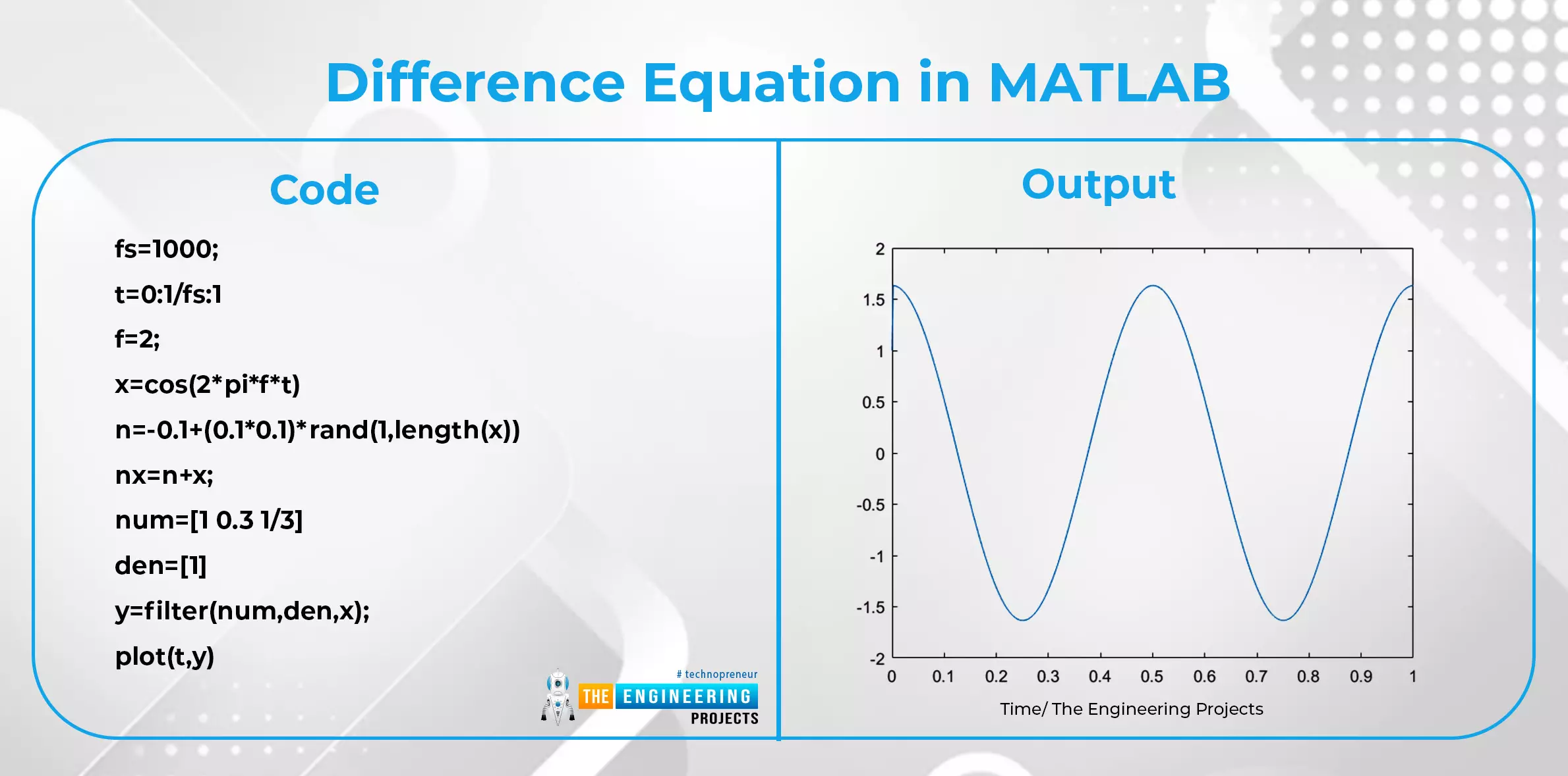
  • What is the difference equation and how is it related to the z transform?

  • What are some important applications of z transform?

We’ll go through each of these topics in detail, so stay with us to learn about all of them.

Properties of z Transform

Till now, we have seen the introduction of z transform along with some basic information. It's time to discuss some properties of z transform in this lecture. We always mention the properties of the topic if possible to clearly describe the nature and workings of that particular topic. It will be correct to say that while discussing the properties of a mathematical tool, we provide you with a wide domain of learning and experimenting about that particular topic. 

Linearity of the z transform

The z transform is always linear. It means, if we have two statements and apply the z transform individually on both of them, then we always get the linear results. Mathematically,

If

 F(z) = Z{fn}

and 

G(z) = Z{gn}

Then

Z{afn + bgn} = aF(z) + bG(z)

Time Shifting Property

When we talk about the time shifting property of z transform, we come to know that while passing through the time shifting process while we are performing the z transform, we get the following results:

 x(n)⟷Z.TX(Z)

If we take n-m instead of n in the property given above, we’ll find the results in which the signal in the z plane multiplies with the z complex number having the exponential power equal to the m with a negative sign with it. 

Time Reversal Property of z Transform

The time reversal property of z transform states that if we have the following condition:

x(n)⟷Z.TX(Z)x(n)⟷Z.TX(Z)

Then after applying the z transform, we will get

x(−n)⟷Z.TX(1/Z)

You can see that after the application of z transform, we get the z in that is present in the denominator of the resultant X value. Therefore, this property is named the reversal property.

Convolution of z Transform

Convolution is an important process in signals and systems and we have also read great detail about it in this course. While merging the concept of convolution and z transform, we get to know that if, 

x(n)⟷Z.TX(Z)x(n)⟷Z.TX(Z)

and 

y(n)⟷Z.TY(Z)y(n)⟷Z.TY(Z)

Then we can easily guess that 

x(n)∗y(n)⟷Z.TX(Z).Y(Z)x(n)∗y(n)⟷Z.TX(Z).Y(Z)

Keep in mind, the convolution is not same as the multiplication of the signal. It is the process in which two signals are overlapped in such a way that they form the third signal that has a mix of the properties of both the signals that are convoluted. 

Corelation of z Transform

If you have studies about the convolution, you will surely have the information of correlation as well. This property of z transform states that if we have 

x(n)⟷Z.TX(Z)x(n)⟷Z.TX(Z)

and 

y(n)⟷Z.TY(Z)

Then after the process of correlation while you are using z transform, you will get the following results:

x(n)⊗y(n)⟷Z.TX(Z).Y(Z−1)

If you are new to the correlation then you must gpo to our previous lecture about correlation where we have descried this briefly. 

Initial Value Theorem

Based on different experiments and studies, a theorem has been introduced and the initial theorem is one of them. This theorem is used to find the initial value of of the statement without using the inverse z transform and it states that:

x(0)=limz→∞X(z)

This theorem is only applicable to casual signals. 

Final Value Theorem

This is another theorem that is usually introduced while discussing the initial value theorem. It states that if:

x(∞)=limz→1[z−1]X(z)

It is also used in cases where you do not want to apply the inverse z transform and use the alternative way.

Z Transform of Unit Impulse Function

The unit impulse function is used in physics and mathematics. It indicates the function that has zero width and a unit area that is the area of value 1. Unit step function using z transform is simple and easy and it results in the sequential series. Suppose we have the following function:

Then after applying the z transform of this statement, we get a geometric series. Recall that geometric series is the one in which every value is the result of the multiplication of the previous value with a particular constant depending upon the condition given for the geometric constant. 

Z transform and Unit Ramp Signal

A unit ramp function is one that after the implementation of different operations, provides a graph that has a straight slope. Such functions are widely used in the formation of complex operations. While using the z transform, it is defined as:

x(n)=r(n)={n For n≥0 0 For n<0 }

Then we can solve this by using the procedure of z transform as:

Multiplication Property of z Transform

The multiplicative property of z transform is also called the complex convolution property of z transform. It is because, it results by the multiplication of two signals of time domain that corresponds to the complex number of z domain. You can have the idea of this property with the help of the code given nex that is the extension of the code that we have worked with before. 


Code

Output 

syms n;

f=sin(2*n)

F=ztrans(f)

G=iztrans(F)

H=F*G

Z Transform and Difference Equation

The difference equation is somehow a special case in the equation and the z transform is used to solve this in an effective way. It is defined as:

“The difference equation is the special type of equation in which there exists a difference (minus operation) of different variables. These show the relationship between an independent variable and the consecutive difference of a dependent variable.

These are not complex equations, and usually they depend upon arithmetic operations. Here is a simple example of the difference equation:

y(n)− 34y(n−1)+y(n−2)=x(n)+x(n−3)

Another example of the difference equation is:

𝒚-(𝒏+𝟐)−𝟔𝒚-(𝒏+𝟏)+𝟗𝒚-𝒏=𝟐^𝒏

There are certain steps that are used to solve the difference equation, and these are given next:

  • Convert the difference equation into the algebraic equation using the specific procedure of the z transform. 

  • Calculate the solution of the resultant equation in the z domain. 

  • Take the time domain equation of the result by using the inverse z transform (that we learned in the previous lecture).

Difference Equation in MATLAB


Code

Output

fs=1000;

t=0:1/fs:1

f=2;

x=cos(2*pi*f*t)

n=-0.1+(0.1*0.1)*rand(1,length(x))

nx=n+x;

num=[1 0.3 1/3]

den=[1]

y=filter(num,den,x);

plot(t,y)


Here, you can see that we have used the plot command to see the signal graphically. You can skip it if you want to have the numerical values only. By changing the frequency value, you can have different types of results. Other parameters that qwe have used are the same that we have described in the previous sections of this series. 

Applications of z Transform

Z transform has great significance in the mathematical field, especially in the signal and system and other branches where the signals have a fundamental role. Till now, we have learned a lot of things about this transform and therefore, we expect that you will understand the reason why this transform is used in almost every field of mathematics. 

Analysis of Digital Filters

As we have said earlier, z transform deals with discrete-time signals. This is the main reason z transform is used in the process of digital filter analysis. The interesting fact is, laplace transform can not be used in this regard because they can not work on the discrete signals. 

The digital filters are the mathematical algorithms that are mainly used in the implemetnatation of digital input signals to obtain the digital output signals.

Analysis of Linear Discrete System

One of the property that we have learned till now is the linearity of z transform and this property is also used in the analysis process of linear discrete system. The are the system that takes the discrete system as input and after different operations, it also restun us the discrete signals again. Z transform is used to maintain the stability of the result throughout the system.

Frequency Response

We all know that the z transform is used to obtain the result in the z plane. It converts the signal with the time domain into other formats, such as the frequency domain. Therefore, while working with the signals, the z transform is used in finding the frequency response. 

Telecommunication

In the field of telecommunication, all systems are based upon the transfer of a number of bits from one place to another. Z transform is used there to stabilize the flow of the bits as they are in the form of discrete signals. Other techniques are also useful for the same purpose, but while using the z transform, it becomes easy to predict the results and the time at which the communication will occur. 

Feedback Control Problems

A Z transform is used to overcome the feedback control problems of the system. It is done by using different types of signals, including continuous time and discrete time signals. This transform can be used differently when practically implemented.

Identification of the Signals

In operations where experts want to know the exponentially changing values of the signals, they prefer to work with the z transform according to the nature of the signal.

Usage of complex number z in z transform

As we have learned previously, there is a z value that is used in the work of z transform. This is an important feature of the z transform because of its complex nature. It is used to perform complex calculations easily, which were not possible with the Laplace transform.

Signal Processing

Z transform is widely used in signal processing ( as we are reading it from the start). Basically, it is a signal processing tool that is efficiently used in the analysis and interaction of different signals. The poles and zeros used in this type of transform help to recognize the nature of the signal; that is, is it casual, stable, or inverse in nature?

It was a long article based upon interesting facts about the z transform. We were having the discussion of the z transform from our previous session where we saw the basics of the z transform. We saw the properties of the z transform and discussed the important points to clarify our concepts. We also use MATLAB for the implementation of a difference equation. In the end, we learned the simple description of the z transforms application to make our minds about the importance of this topic. If you want to learn more, you can find examples of each property and Use them as your homework. The next lecture is also going to be a little bit complex yet interesting because we are going to learn another transform, which is the Fourier transform.

Introduction to Z Transform in Signal and Systems with MATLAB

Hey learners! Welcome to another exciting lecture in this series of signals and systems. We are learning about the transform in signals and systems, and in the previous lectures, we have seen a bulk of information about the Laplace transform. If you know the previous concepts of signal and system, then this lecture will be super easy for you to learn, but if your concepts are not clear, do not worry because we will revise all the basic information from scratch for our new readers. So, without wasting time, have a look at the topics of today.

  1. What is z transform? 

  2. What is the region of convergence of z transform?

  3. What are some of the important properties of the region of convergence?

  4. How to solve the z transform?

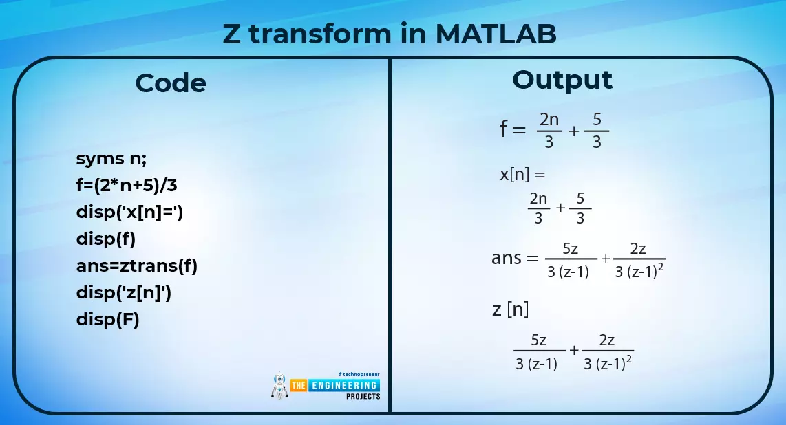
  5. What is an example of the z transform in MATLAB?

  6. What are the methods for the inverse z transform?

What is z transform?

You must have an idea that the Laplace transform is a general case transform and converts the signal from a time domain into a frequency domain. The same is the case with the z transform, it changes the domain of the signal but in another way. The Laplace transform is associated with the power signal and the z transform has some other characteristics. Usually, the z transform is used to understand the stability of the system. Z transforms are used in

  • Energy signals

  • Power signals

  • Neither power nor energy signals

Yet it is applicable to a certain level, and after that level, it is not that much more effective. The Z transform is a powerful mathematical tool and is widely used in mathematical courses and applications including signals and systems. We introduce the z transform as:

"The Z transform is a mathematical tool that, after different procedures, converts the differential equation (with time domain) into the algebraic equation of the z domain."

Mathematically, we show it as:

As you can see clearly, the summation sign contains the limits from negative infinity to positive infinity which means it is a bilateral function of the z transform that we have shared with you. 

By the same token, you can also predict that the z transform also has another region that lies between the zero to positive infinity. It is called the unilateral z transform and it works a little bit differently than the first case discussed here. We describe it as:

Let’s discuss the whole statement in detail but prior to starting, recall in your mind the definition of discrete-time signals. We know that:

“A discrete-time signal is one whose value can be measured at discrete intervals." When working with a discrete-time signal, there will be time intervals of n during which you will not have a value. In the representation of DT signals, the form x[n] is used. Discrete signals approximate continuous-time (CT) signals."

Therefore, when talking about the z transform, keep the definition of z transform in your mind to understand what exactly is going on. 

Now, look at the statement given above.

  • We have the discrete-time signal in the time domain represented by x[t]. 

  • We applied the z transform to it. 

  • Now, we got the same signal that lies in the z domain and is multiplied with a complex number z having the exponential of the n with a negative sign. 

  • Do not worry about the value of n all the time. The summation sign indicates that the value of n starts from negative infinity (or zero in unilateral z transform) to positive infinity, and in this way, we found the values of the series. (This will be much clearer when we discuss the procedure).

    Here z is a complex number that is described with the help of this equation:

    At this level, there is no need to describe the basic concepts of complex numbers. In general, we can summarize the above discussion through the statement given next:

    x(n)⟷X(Z)

    The whole discrete time signal is converted into another format with the z transform as a base,

    Region of Convergence of z Transform

    The region of convergence, or simply ROC, is an important term that is used to describe the range of z in the z transform. As we have said, z is a complex number and its range, therefore, has different types of properties. 

    Properties of the Region of Convergence

    • No. of poles: In z transform, where x[z] is always finite, there are no poles. (We’ll define them in a later section). The ROC of the z transform does not contain any poles. 

    • When talking about a right-sided signal, the region of convergence is always outside the z-plane circle.

    Where the shaded area is ROC.


    • When talking about a left-sided signal, the region of convergence is always inside the z-plane circle.

    Where the shaded area is ROC.

    • If we have the signal on both sides, then the region of ROC is in the form of a ring inside the circle. 

    • To have a stable form, the region of convergence has a unit value.

    Procedure to Solve z Transform

    There are different cases in the z transform that if we start to describe, will be more confusing and time taking than other transforms. So, we’ll discuss a general format of z transform, and after practice, you will learn the procedure effectively. 

    Thoroughly examine the question. 

    Use the formula of the z transform given above.

    • Put z into the denominator as it has negative power. Doing so will convert the negative power into a positive. 

    • Make sure you take the common values out of the sequence. 

    • Put the value of n as 0, 1, 2, 3, 4, and so on to get the series. 

    • Solve the equation.

    It is the most basic and simple description, but the z transform is not that simple. Instead of solving the long calculations, why not use MATLAB for practical implementation? If you have your own course instructor at university, you must have the idea of solving the procedure by hand. 

    Z transform in MATLAB

    In MATLAB, the z transform is as simple as the previous transform was. Therefore, we are emphasizing the usage of MATLAB at every step. Note that if you want to have a detailed procedure to perform the functions theoretically, you can find your instructors. But from the performance point of view, you should go to MATLAB to confirm your answers all the time. Here is a simple example of an equation that also shows some little details. 

    Code:

    syms n;

    f=(2*n+5)/3

    disp('x[n]=')

    disp(f)

    ans=ztrans(f)

    disp('z[n]')

    disp(F)


    Output:

    Here, you can see we have used the pre-defined function of z transform given as:

    ztrans(x)

    With the help of the z transform, you can solve any equation or expression that you want. 

    Notice that we have used a display function in the code. You must know that z transform can also be done in MATLAB without using the function. 

    Display function in MATLAB

    The display function is used to label the numerical output. It does the same work as the xlabel and ylabel in the graphical window of MATLAB. Moreover, this function is also used to call the value that we have specified before using it and to display the results directly. The syntax of the display function is

    1. disp(x)

    2. disp(‘x’)

    Where,

    • To display the string value, we use inverted commas around the value. 

    • To call the value of x, we simply use it as it is. 

    • Never use this function with a capital D or any other change in the spelling, otherwise, you will get the error. 

    Have a look at another example of the z transform in which we added two trigonometric functions and found their z transform.

    Code:

    syms n;

    f=sin(2*n)

    ans=ztrans(f)

    g=cos(3*3.14*n)

    ans=ztrans(g)

    Output:

    Zaros and poles of z transform

    When you study this particular topic of z transform, you will hear some terms named as zeros and poles. These are the simple topics while learning z transform and usually, are used in the numerical problem. Consider the following equation:

    Zeros: while solving the equation with the fraction, the numerator contains the M roots corresponding to the zeros. In the equation given above, q represents the zeros.

    Poles: When you are solving the fractional equation by z transform, the N roots in the denominator are called the poles. Here, these are represented with the letter p.

    While solving the z transform, we make a circular representation to solve the equation, just like we did while we were learning ROC. Poles are represented at the y-axis, and zeros are represented at the x-axis.

    Inverse z Transform

    As you can guess from the name, the inverse z transform is used to convert the results of the z transform into the form before the z transform. There are different methods through which the calculations of the z transform are inverted from an equation. 

    1. Long division 

    2. The partial fraction method of inverse z transforms

    3. Residue method

    4. Power series of inverse z transform

    Long Division Method 

    This method is applicable when:

    • There is a ratio of two polynomials

    • The polynomials can not be factorized

    To apply inverse z transform with this method, the division process of numerator with denominator is carried out. The resultant equation is then passed through the procedure of inverse z transform and we get the results. It is a complex method. 

    Partial Fraction Method of Inverse z Transform

    This is the method that involves the rules and procedure of partial fraction (we have received it in the previous lecture) and after that, the inverse z transform is applied. 

    Residue Method

    There are different names for this method including the inversion integration method and contour integral method. For this method, we have to follow the equation given below:

    The inverse z transform is obtained by summing up all the residues of this equation from the poles point of view.

    Power Series of Inverse z Transform

    In the end, this is the simplest and easiest way to find the z transform. In this method, the equation is expanded and we get the series of ascending powers. After that, the coefficient of z^-n is the required result. 

    Inverse z transform in MATLAB 

    To apply the inverse z transform in MATLAB, we use the following formula:

    iztrans(x)

    For convenience, we have put the process of z transform and the inverse in the same code. 

    Code:

    syms n;

    f=sin(2*n)

    F=ztrans(f)

    G=iztrans(F)

    Output:

    You can clearly see that we got our required result easily. This type of transforms is used when the data is being transferred to different networks. There are many applications of this transform and you will learn about them in the next section. 

    We have started the discussion of another transform named the z transform that is somehow similar to the Laplace transform that we have learned in the previous sessions. Z transform is a useful mathematical tool and we studied the ROC, procedure, and the inverse method of z transform. We also saw some examples in MATLAB. In the next lecture, we are going to learn some other basic information on the same topic.

    Syed Zain Nasir

    I am Syed Zain Nasir, the founder of <a href=https://www.TheEngineeringProjects.com/>The Engineering Projects</a> (TEP). I am a programmer since 2009 before that I just search things, make small projects and now I am sharing my knowledge through this platform.I also work as a freelancer and did many projects related to programming and electrical circuitry. <a href=https://plus.google.com/+SyedZainNasir/>My Google Profile+</a>

    Share
    Published by
    Syed Zain Nasir