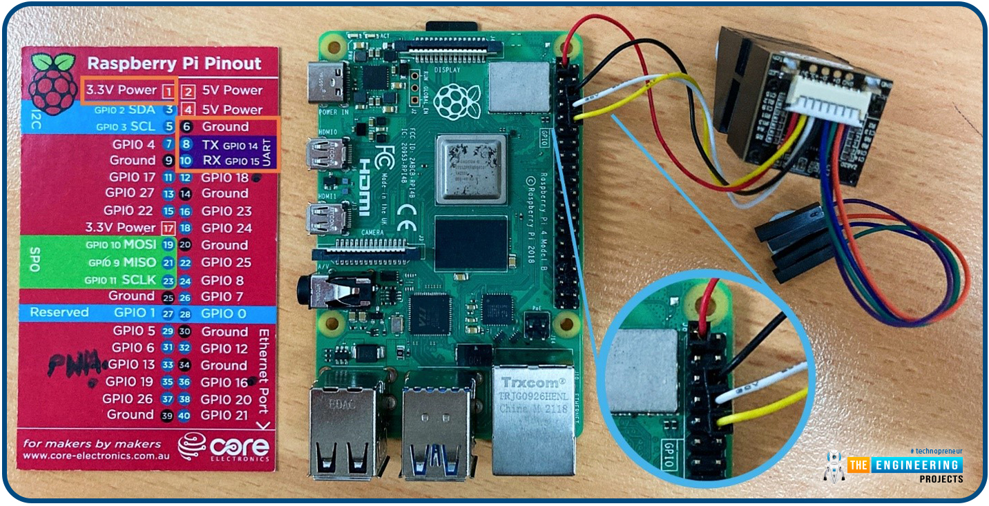
Thank you for joining us today for our in-depth Raspberry Pi programming tutorial. The previous guide covered the steps necessary to connect a fingerprint scanner to a Raspberry Pi 4. In addition, we developed a python script to complement the sensor's ability to identify fingerprints. Yet, in this guide, we'll discover how to interface a ws2812 RGB to a Raspberry Pi 4.
Bright, colorful lights are the best, and this tutorial shows you how to set up Fully Configurable WS2812B led strips to run on a Pi 4 computer as quickly and flexibly as possible. In that manner, you can have the ambiance of your home reflect your tastes.
In most cases, when people talk about a "WS2812B Strip," they mean a long piece of extensible PCB with a bunch of different RG ...
Hello friends, I hope you all are going great. Today, I am going to share the 10th tutorial of Section-III in our Raspberry Pi Programming Course. In our previous tutorial, we interfaced a Gas Sensor MQ-2 with Raspberry Pi 4. Today, we will be interfacing a Fingerprint Sensor with Raspberry Pi today.
After appearing only in science fiction films until recently, fingerprint sensors are often employed to confirm an individual's identity in various contexts. Today, fingerprint-based systems are used for everything from checking in at the office to verifying an employee's identity at the bank, withdrawing cash from an ATM, and proving one's identity at a government agency. For identifying purposes, fingerprint-detecting technology has been used for so ...
We all know technology is not only changing trends and habits, but it is also reshaping the way we live our daily lives. We are not talking about centuries ago, but even if we examine the previous two decades, everything, from our communication style to our travel means, from our shopping habits to our entertainment industry, is changing rapidly, and this has both pros and cons. In a broader view, we can say that positive impacts are more dominant than negative effects on our lives. Maybe you have the opposite opinion, but I can prove this with the help of a simple and general example that I am going to discuss in detail with you. Just like almost every other sport and game, poker has some visible technical changes, and people can play poker online. Clients and casinos are getting more and ...
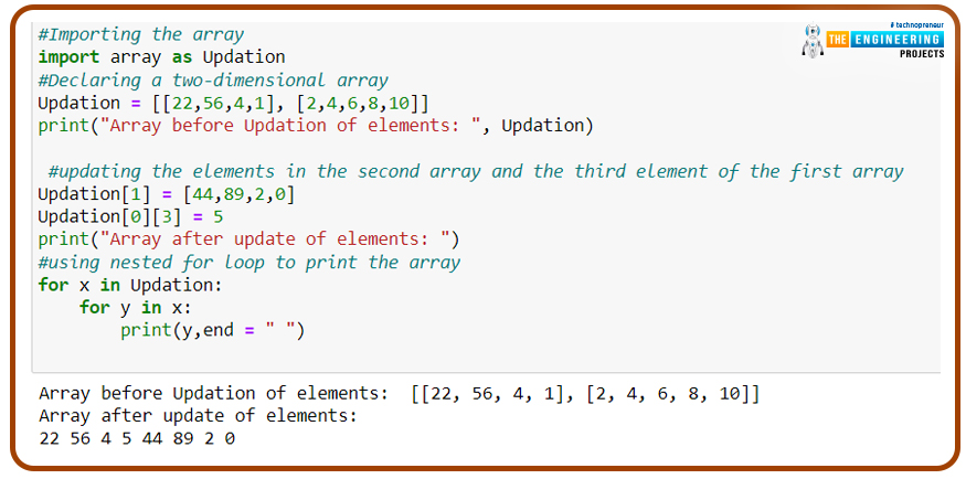
Hello learners! Welcome to the next episode of the arrays, in which we are moving towards the details of the arrays at an advanced level. In the previous lecture, we covered the introductions and fundamentals of arrays, dimensional arrays, and array operations. One must know that the working of the arrays does not end with simple operations, and there is a lot to learn about them. Arrays and their types are important topics in programming, and if we talk about Python, the working and concepts of the array in Python are relatively simple and more effective. The details of the advanced types of arrays will prove this statement. We have a lot of data to share with you, and for this reason, we have arranged this lecture. It is important to understand the reasons behind the reading of this lect ...
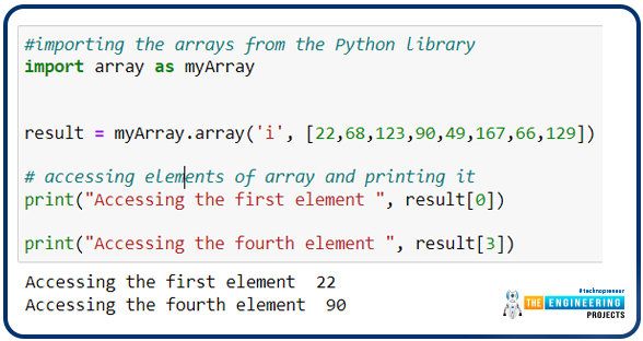
Hello Python programmers! Welcome to the engineering projects where you will find the best learning data in a precise way. We are dealing with Python nowadays, and today, the topic of discussion is the arrays in the language. We have seen different data types in Python and discussed a lot about them in detail till now. In the previous lecture, we saw the details of the procedures in dictionaries. There are certain ways to store the data in the different types of sequences, and we have highlighted a lot about almost all of them. It is time to discuss the arrays, but before this, it is better to understand the objectives of this lecture:
Introduction to arrays
Difference between contiguous and non-contiguous memory locations
One-dimensional arrays
Functions in arrays
What are Arra ...
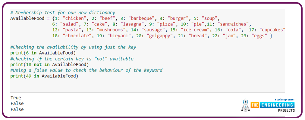
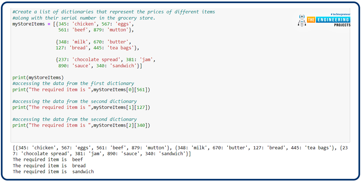
Hello peeps! Welcome to the new episode of the Python tutorial. We have been working with different types of data collection in Python, and it is amazing to see that there are several ways to store and retrieve data. In the previous lecture, our focus was on the basics of dictionaries. We observed that there are many important topics in the dictionaries, and we must know all of them to make our base of concepts solid. For this, we are now dealing with the dictionaries in different ways, and this tutorial is going to be very interesting because we will pay more heed to the practical work and, by choosing a few cases in our codes, we will apply multiple operations to them. So have the highlights of today’s learning, and then we will move forward with the concepts.
What are nested diction ...
Hello students! Welcome to the new Python tutorial, where we are learning a lot about this programming language by applying the codes in a Jupyter notebook. It is interesting to see how simple codes with easy syntax can be useful to store, retrieve, and use data in different ways. Many things in Python are so unadorned and pre-defined that programmers may use them in a productive way without any issue.
In the previous lecture, we have seen the details of the sets and how different types of mathematical operations are used to get the required results. We have seen many codes, the examples of which were taken from day-to-day life. In the present lecture, the mission is to learn a new topic that is related to the concepts of previous lectures. Yet, it is important to have a glance at t ...
Online technology has had a profound impact on the real world, revolutionizing various industries and areas of our lives. From e-commerce and communication to education, healthcare, and entertainment, online technology has made many aspects of daily life more convenient, accessible, and efficient.
This technology has fundamentally changed the way people interact with the world around them — and there is no denying — another industry that has been significantly transformed by online technology is — the gaming industry.
With the rise of Live casino online technology
and advancements in internet connectivity, players can now connect and compete with others from anywhere in the world. Online technology has also enabled the development of massively multiplayer online games (MMOs) that allow ...
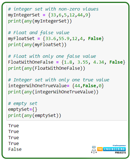
Hey people! Welcome to another tutorial on Python programming. We hope you are doing great in Python. Python is one of the most popular languages around the globe, and it is not surprising that you are interested in learning about the comparatively complex concepts of Python. In the previous class, our focus was to learn the basics of sets, and we saw the properties of sets in detail with the help of coding examples. We found it useful in many general cases, and in the present lecture, our interest is in the built-in functions that can be used with the sets. Still, before going deep into the topic, it is better to have a glance at the following headings:
What are the built-in functions?
How do we perform the all() function with examples?
What is the difference between any() and all()? ...
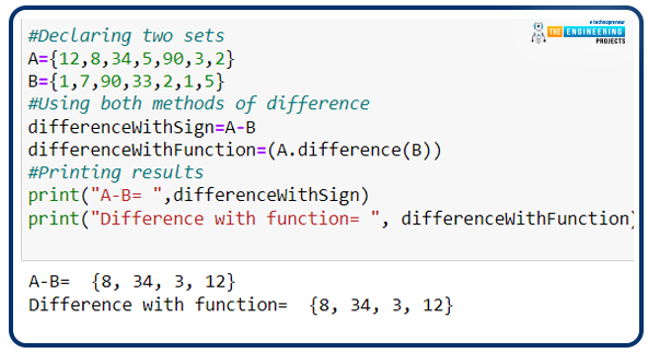
Hey, learners! Welcome to the next tutorial on Python with examples. We have been working with the collection of elements in different ways, and in the previous lecture, the topic was the built-in functions that were used with the sets in different ways. In the present lecture, we will pay heed to the basic operations of the set and their working in particular ways. We are making sure that each and every example is taken simply and easily, but the explanation is so clear that every user understands the concept and, at the same time, learns a new concept without any difficulty. The discussion will start after this short introduction of topics:
How do we declare and then find the difference between the two sets?
What are the built-in functions for operations, and how do we use them in the ...