Online technology has had a profound impact on the real world, revolutionizing various industries and areas of our lives. From e-commerce and communication to education, healthcare, and entertainment, online technology has made many aspects of daily life more convenient, accessible, and efficient.
This technology has fundamentally changed the way people interact with the world around them — and there is no denying — another industry that has been significantly transformed by online technology is — the gaming industry.
With the rise of Live casino online technology
and advancements in internet connectivity, players can now connect and compete with others from anywhere in the world. Online technology has also enabled the development of massively multiplayer online games (MMOs) that allow ...
Hey people! Welcome to another tutorial on Python programming. We hope you are doing great in Python. Python is one of the most popular languages around the globe, and it is not surprising that you are interested in learning about the comparatively complex concepts of Python. In the previous class, our focus was to learn the basics of sets, and we saw the properties of sets in detail with the help of coding examples. We found it useful in many general cases, and in the present lecture, our interest is in the built-in functions that can be used with the sets. Still, before going deep into the topic, it is better to have a glance at the following headings:
What are the built-in functions?
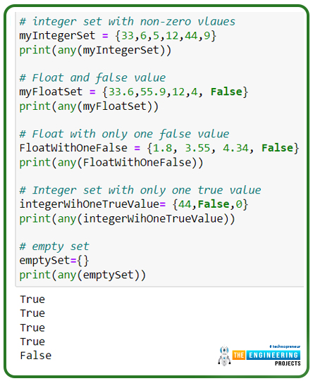
How do we perform the all() function with examples?
What is the difference between any() and all()? ...
Hey, learners! Welcome to the next tutorial on Python with examples. We have been working with the collection of elements in different ways, and in the previous lecture, the topic was the built-in functions that were used with the sets in different ways. In the present lecture, we will pay heed to the basic operations of the set and their working in particular ways. We are making sure that each and every example is taken simply and easily, but the explanation is so clear that every user understands the concept and, at the same time, learns a new concept without any difficulty. The discussion will start after this short introduction of topics:
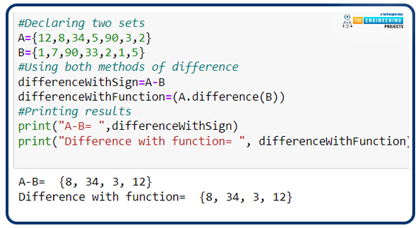
How do we declare and then find the difference between the two sets?
What are the built-in functions for operations, and how do we use them in the ...
Writing an essay is a critical skill that every student must learn.
It’s not an easy task, I understand.
But with deliberate practice and careful attention you can learn to write an essay like a pro.
Essays serve as a vital tool for academic and personal development, allowing individuals to express their thoughts, opinions, and arguments in a structured and coherent manner.
Whether you are writing a college application essay, a research paper, or a personal narrative, the ability to communicate your ideas effectively is essential.
Needless to say, the job of writing an essay can seem daunting, especially if you are a beginner. This guide aims to provide you with a comprehensive overview of the essay writing process, from preparing to write to formatting and fin ...
Although 3D printing feels like a relatively new development, there are lots of promising projects underway. A scheme to build 46 eco-homes has been approved in the UK’s first 3D printed development
, for example, and the same is happening in Australia to provide housing for remote indigenous communities in rural areas
.
But how can 3D printing be applied in business? Here’s a breakdown on how it can be used and the opportunities it creates.
What is 3D printing?
3D printing refers to technology that can form materials using computer designs. The earliest signs of 3D printing came about in 1981. Dr. Hideo Kodama created a rapid prototyping machine that built solid parts using a resin and a layer-by-layer system.
Using a bottom-up technique, the material is layered until a tangib ...
Artificial intelligence is becoming more and more important for data security. In this post, we'll look at how AI may assist businesses in anticipating and thwarting threats. But before going ahead we will explain the terms artificial intelligence and machine Learning.
What Is Artificial Intelligence
Artificial intelligence (AI) is a discipline of computer science that focuses on making electrical equipment and software intelligent enough to do human activities. AI is a broad concept and a basic subject of computer science that may be used to a variety of domains including learning, planning, problem solving, speech recognition, object identification and tracking, and other security applications.
Artificial intelligence is divided into n ...
Hi Everyone! How are you doing, my friends? Today I bring a crucial topic for PLC programmers, technicians and engineers. We have been working together for a long time using ladder logic programming. We have completed together dozens of projects from real life and industry. One day I was thinking about what we have done in this series of ladder logic programming, and I came across that I missed talking about one essential topic ever. You know what? It’s the PLC troubleshooting and online debugging! After writing a ladder logic program for the project, you can imagine it should operate from the download moment 24/7. As usual, any system goes faulty one day. So we need to go through this matter, showing you how to find our PLC faults, troubleshoot, and go online with the PLC to figure out th ...
Hi, my friends and welcome back. I am happy to meet you again with a new tutorial of our PLC ladder logic programming series tutorials. Today we will complete what we started the last tutorial on the Elevator control project. We have a bunch of duties to complete together today. So let’s save time and jump into work immediately.
Project description:
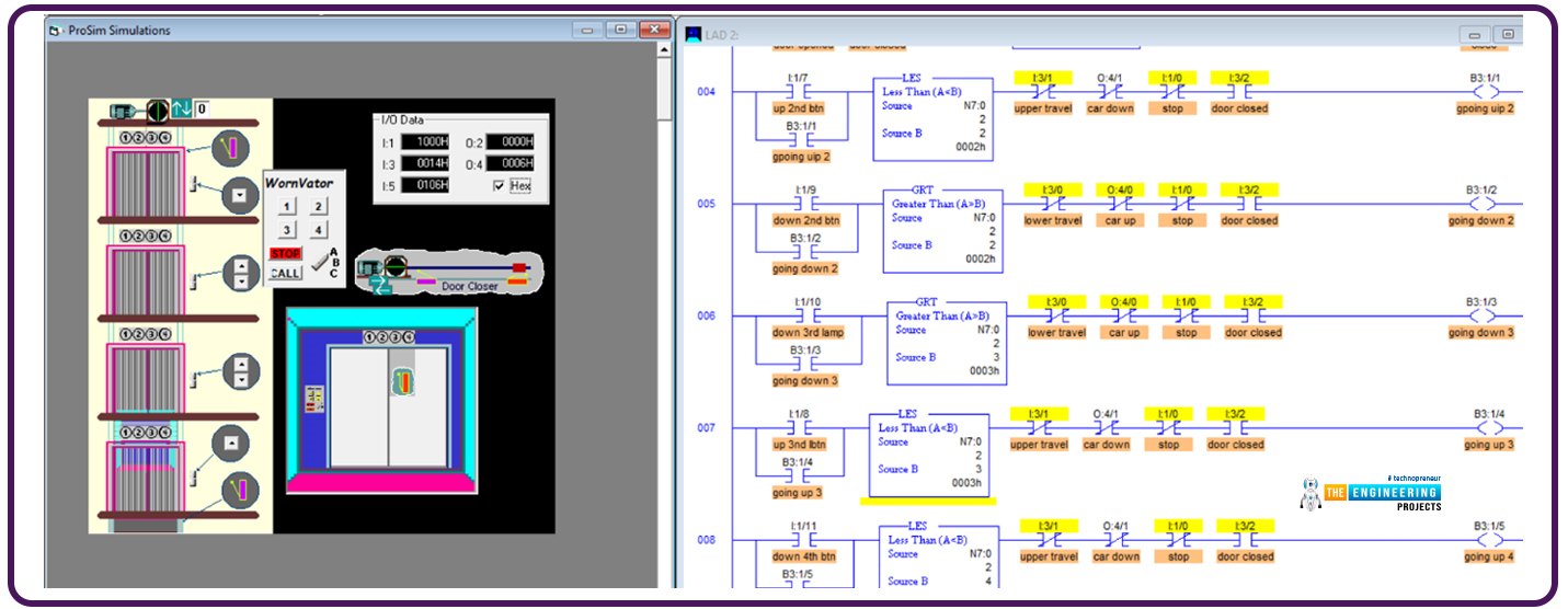
Figure one shows the details that might help me describe the project between our hands. We have an elevator car that travels up and down and can stop on one of four floors based on the passengers’ requests. We have 6 push buttons on the wall next to the elevator door that can send requests to call the elevator. In addition, there is a control panel inside the elevator cabinet in which there are push buttons to request stations to reach floors ...
Hello, my friends and welcome back with one new tutorial of our ladder logic programming series. Today I am bringing one exciting project which you can see everywhere, in your home, work, and public places, which is an elevator. We will design a solution using plc ladder logic programming, which drives the elevator. Our elevator is composed of 4 floors and has all capabilities of large-scale elevators. So let’s get started and save time and jump into our tutorial.
Elevator Project
As you can see, Everyone figure 1 depicts the complete scene of the project and tells that the elevator we will manage has four floors to visit. On the first floor, there is only one outer request to call the car from any floor above, i.e. from floor 2, floor 3, or floor 4. While on the second floor, there are ...
Hello everyone, and welcome back with a new tutorial in our ladder logic programming. Today we will continue the bottle line production line using ladder logic programming. Let me remind you, everyone; we have seen how to utilize the bit shift left instruction BSL to save the data that describes the state of a bottle, including the present state, size state, either large or small size and the excellent and broken state as well. And also we utilized these states to energize the large bottle and scrap solenoid to divert the bottles to the appropriate position and conveyor. At the end of the day, we have separated small, large, and scrap bottles. Today we are going to manage the scraping of the broken bottle.
Bottle line Scraping management
In each bottle line process, we have a common and ...