Autoencoders as Masters of Data Compression

Hey readers! Welcome to the next episode of training on neural networks. We have been studying multiple modern neural networks and today we’ll talk about autoencoders. Along with data compression and feature extraction, autoencoders are extensively used in different fields. Today, we’ll understand the multiple features of these neural networks to understand their importance.

In this tutorial, we’ll start learning with the introduction of autoencoders. After that, we’ll go through the basic concept to understand the features of autoencoders. We’ll also see the step by step by step process of autoencoders and in the end, we’ll see the model types of autoencoders. Let’s rush towards the first topic:

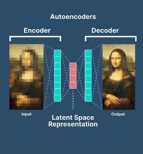
What are Autoencoders?

Autoencoders are the type of neural networks that are used to learn the compressed and low-dimensional representation of the data. These are used for unsupervised learning and are particularly used in tasks such as data compression, feature learning, generation of new data, etc. These networks consist of two basic parts:

  1. Encoders

  2. Decoders

Moreover, between these two components, it is important to understand the latent space that is sometimes considered the third part of the autoencoders. The goal of this network is to train and reconstruct the input data at the output layer. The main purpose of these networks is to extract and compress the data into a more useful state. After that, they can easily regain the data from the compressed state.

Basic Concepts to Understand Autoencoders

The following are some important points that must be made clear when dealing with the autoencoder neural network: 

Encoders in Autoencoder Neural Network

This is the first and most basic component of the autoencoders. These are considered the heart of autoencoders because they have the ability to compress and represent the data. The main focus of encoders is to map the input data from high dimensional space to low dimensional space. In this way, the format of the data is changed to a more usable format. In other words, the duty of encoders is to distill the essence of the input data in a concise and informative way.

Autoencoders Latent Space

The output of the autoencoders is known as latent space. The difference between the latent space and the original data is given here:

Dimensions of Data

The dimension of the data is an important aspect of neural networks. Here, the dimensions are smaller and more compact than in the original data. Choosing the right dimension is crucial for efficient representation and detail in getting the details of the data.

Structure of the Latent Space

The structure of the data from encoders (latent space) has information about the relationship between data points. These are arranged in such a way that similar data points are placed closer to each other and dissimilar data points are far apart. This type of spatial arrangement helps in the efficient retrieval and arrangement of the data in a more efficient way. 

Feature Extraction in Latent Space

Feature extraction is an important point in this regard because it is easier with the latent space data than with the normal input data fed into the encoders. Hence, feature extraction is made easy with this data for processes like classification, anomaly detection, generating new data, etc. 

Decoders in Autoencoders

The decoder, as the name suggests, is used to regenerate the original data. These take the data from the latent space and reconstruct the original input data from it. Here, the pattern and information in the latent space are studied in detail and as a result, closely resembling input data is generated. 

Generally, the structure of encoders is the mirror image of the encoders in reverse order. For instance, if the architecture of the encoders has convolutional layers, then the decoders have deconvolution layers.

During the training process, the decoder’s weight is adjusted Usually, the final layer of the decoders resembles the data of the initial layer of the input data in the encoders. It is done by updating and maintaining the weights of the decoders corresponding to the respective encoders. The difference is that the neurons in the decoders are arranged in such a way that the noise in the input data of the encoders can be minimized. 

Steps in the Training Process of Autoencoders

The training process for the autoencoders is divided into different steps. It is important to learn all of these one by one according to the sequence. Here are the steps:

Data Preparation in Autoencoders

The data preparation is divided into two steps, listed below:

Gathering of the Data 

The first step is to gather the data on which the autoencoders have to work. For this, a dataset related to the task to be trained is required. 

Autoencoders Preprocessing

The preparation of the data required initial preprocessing. It requires different steps, such as normalization, resizing for images, etc. These processes are selected based on the type of data and the task. At the end of this process, the data is made compatible with the network architecture.

Autoencoders Model Architecture

There are multiple architectures that can be used in autoencoders. Here are the steps that are involved in this step:

Selecting the Appropriate Architecture

It is very important to select the right architecture according to the datasets. The encoder architecture aligns with the data type and requirements of the task. Some important architectures for autoencoders are convolutional for images and recurrent for text.

Autoencoders Network Layers Specifications

In the same step, the basic settings of the network layers are also determined. Following are some basic features that are determined in this step:

  • Determination of the number of layers in the network

  • Numbers of neurons per layer

  • Suitable activation functions according to the data (e.g., ReLU, tanh).

Autoencoders Training Loops

The training is the most essential step and it requires great processing power. Here are the important features of the autoencoders:

Autoencoders Feed Forward

In this step, the processing of the input data is carried out. The data is sent to the encoder layer, which generates the latent representation. As a result of this, latent space is generated. 

Decoder Reconstruction

The latent space from the encoder is then sent to the decoder for the regeneration of the input data, as mentioned before. 

Autoencoders Output Calculation 

Here, the decoders’ output is then calculated with the original input. Different techniques are used for this process to understand the loss of data. This step makes sure that the accurate data loss is calculated so that the right technique is used to work on the deficiencies of the data. For instance, in some cases, the mean squared error for images is used and in other cases, categorical cross-entropy for text is used to regenerate the missing part of the data. 

Autoencoders Backpropagation 

Backpropagation is an important process in neural networks. The network propagates backward and goes through all the weights to check for any errors. This is done by the encoders as well as by the decoders. The weights and bosses are adjusted in both layers and this ensures the minimum errors in the resultant networks.

Autoencoders Optimization

Once the training process is complete, the results obtained are then optimized to get an even better output. These two steps are involved here:

Choosing the Right Optimizer

Different cases require different types of calculations; therefore, more than one type of optimizer is present. Here, the right optimizer is used to guide the weight update. Some famous examples of optimizers are Adam and stochastic gradient descent. 

Autoencoders Learning Rate Adjustment

Another step in the optimization is the learning rate adjustment. Multiple experiments are done on the resultant output to control the learning speed and avoid overfitting the data in the output. 

Autoencoders Regulation

This is an optional step in the autoencoders that can prevent overfitting. Here, some different techniques, such as dropout and weight decay, are incorporated into the model. As a result of this step, the training data memorization and improvement of the generalization of the unseen data are seen. 

Autoencoder Monitoring and Evaluation

The getting of the results is not enough here. Graduation monitoring is important for maintaining the outputs of the neural networks. Two important points in these steps are explained here:

Tracking Training Process

During the training process, different matrices are assessed to ensure the perfect model performance; some of these are given here:

  • Monitor reconstruction loss

  • Checking for the accuracy of results

  • Checking the rate of precision

  • Recalling the steps for better performance

The evaluation process is important because it ensures that any abnormality in the processing is caused during its initial phase. It stops the training process to prevent any overfitting of the data or any other validation. 

Autoencoders Models 

The autoencoders have two distinct types of models that are applied according to the needs of the task. These are not the different architectures of the data but are the designs that relate to the output in the latent space of the autoencoders. The details of each of these are given here:

Under-complete Autoencoders

In under-complete autoencoders, the representation of the latent space dimensions is kept lower than the input space. The main objective of these autoencoders is to force the model to learn all the most essential features of the data that are obtained after the compression of the input. This results in the discovery of efficient data representation and, as a result, better performance.

Another advantage of using this autoencoder is that it only captures the rare and essential features of the input data. In other words, the most salient and discriminative data is processed here. 

Dimensionality Reduction in Under-complete Autoencoders

The most prominent feature of this autoencoder is that it reduces the dimensions of the input data. The input data is compressed into a more concise way but the essential features are identified and work is done on them.

Under Complete Autoencoders Applications

The following are important applications of this model:

  • The main use for an under-complete autoencoder is in cases where compression of the data is the primary goal of the model. The important features are kept in compressed form and the overall size of the data is reduced. One of the most important examples in this regard is image compression. 

  • These are efficient for learning the new representation of the efficient data representation. These can learn effectively from the hierarchical and meaningful features of the data given to them. 

  • Denoising and feature extraction are important applications of this autoencoder. 

Over Complete Autoencoders

In over-complete autoencoders, the dimensions of the latent space are intentionally kept higher than the dimensions of the latent space. As a result, these can learn more expressive representations of the data obtained as a result. This potentially captures redundant or non-essential information through the input data. 

This model enables the capture of the variation in the input data. As a result, it makes the model more robust. In this case, redundant and non-essential information is obtained from the input data. This is important in places where robust data is required and the variation of the input data is the main goal. 

Feature Richness 

The special feature of the autoencoder is its feature richness. These can easily represent the input data with a greater degree of freedom. More features are obtained in this case that are usually ignored and overlooked by the undercomplete autoencoders. 

Applications of Overcomplete Autoencoders

The main applications of overcomplete autoencoders are in tasks where generative tasks are required. As a result, new and more diverse samples are generated. 

Another application to mention here is representation learning. Here, the input data is represented in a richer format and more details are obtained.

Hence, today, we have seen the important points about the autoencoders. At the start, we saw the introduction of the autoencoders neural networks. After that, we understood the basic concepts that helped a lot to understand the working process of autoencoders. After that, we saw the step-by-step training of the autoencoders and in the end, we saw two different models that are adopted when dealing with the data in autoencoders. We saw the specific information about these types and understood the features in detail. I hope this is now clear to you and this article was helpful for you.

Echo State Networks (ESNs) | Working, Algorithms & Applications

Hello pupils! Welcome to the next section of neural network training. We have been studying modern neural networks in detail, and today we are moving towards the next neural network, which is the Echo State Network (ESN). It is a type of recurrent neural network and is famous because of its simplicity and effectiveness. 

In this tutorial, we’ll start learning with the basic introduction of echo state networks. After that, we’ll see the basic concepts that will help us to understand the work of these networks. Just after this, we’ll see the steps involved in setting the ESNs. In the end, we’ll see te fields where ESNs are extensively used. Let’s start with the first topic:

Introduction to Echo State Networks (ESNs)

The echo state networks (ESNs) are a famous type of reservoir computer that uses recurrent neural networks for their functionalities. These are modern neural networks; therefore, their working is different from the traditional neural networks. During the training process, this does not rely on the randomly configured "reservoir" of neurons instead of backpropagation, as we observe in traditional neural networks. In this way, they provide faster and better performance. 

The connectivity of the hidden neurons and their weights are fixed and these are assigned randomly. This helps it provide temporal patterns. These networks have applications in signal processing and time-series prediction.  

Basic Concepts of Echo State Networks (ESNs)

Before going into detail about how it works, there is a need to clarify the basic concepts of this network. This not only clarifies the discussion of the work but will also clarify the basic introduction. Here are the important points to understand here:

Reservoir Computing in ESN

The basic feature of ESN is the presence of the concept of computing reservoir. This is a hidden layer that has randomly distributed neurons. This random distribution makes sure that the input data is captured by the network effectively and does not overfit the specific pattern as is done in some other neural networks. In simple words, the reservoirs are known as the randomly connected recurrent network because of their structure. These reservoirs are not trained but play their role randomly in the computing process. 

Comparing RNN with ESN

ESNs are members of a family of recurrent neural networks. The working of ESNs is similar to RNN but there are some distinctions as well. Let us discuss both:

  • The RNN is a class of artificial neural networks that use sequential and temporal data for their work. The ESN has the same working principle; therefore, it can also maintain the memory of past responses.
  • During the processing of RNN as well as the ESN, the order of the input elements affects the output.
  • Both of these have long-term and short-term dependencies within the sequence; therefore, the role of sequence in these networks is important.

Now, here are some differences between these two:

ESN vs. RNN

The difference between the training approaches of both of these is given here:

  • In the training process of RNN, all the work is done with backpropagation. This causes problems in the vanishing and exploding gradients. The ESNs have a fixed random recurrent weight matrix therefore, the structure is quite simpler than RNN because, here in the training, only output weights are adjusted.
  • In RNN, all the weights, including the recurrent connections, are trainable. Whereas, in ESNs, the reservoirs are not only fixed but are randomly assigned during the process of initialization. During the processing, the calculations are done only with the neurons that are connected to the reservoirs. This not only makes it less complex but also lessens the processing time.
  • In RNNs, the neurons in the network are fully connected but in ESNs, the concept of sparsity is present. According to this concept, each neuron is connected to a subset of the other neuron only. This makes the ESN more productive and simple.

Echo State Property in ESN

The ESN has a special property known as echo state property or ESP. According to this, the dynamics of the reservoirs are set in such a way that they have the fading memory of the past inputs. That means the structure of these neural networks must be created in such a way that it pays more attention to the new input concerning the memory. As a result, the old inputs will fade from memory with time. This makes it lightweight and simple. 

Non-linear Activation Function in ESN

In ESNs, the reservoir’s neurons have a non-linear activation function; therefore, these can deal with complex and nonlinear input data. As mentioned before, the ESNs employ fixed reservoirs that help them develop dynamic and computational capabilities. 

How Do Echo State Networks Work?

Not only the structure, but the working of the ESNs is also different from that of traditional neural networks. There are several key steps for the working of the ESNs. Here is the detail of each step:

Initialization in ESNs

In the first step, the initialization of the network is carried out. As we mentioned before, there are three basic types of layers in this network, named:

  1. Input layer
  2. Reservoir layer (hidden layer)
  3. Output layer

This step is responsible for setting up the structure of the network with these layers. This also involves the assignment of the random values to the neuron weights. The internal dynamics of the reservoir layers evolve as more data is collected in these layers.

Usage of Echo State Property 

The echo state property of ESNs makes them unique among the other neural networks. Multiple calculations are carried out in the layers of the ESNs, and because of this property, the network responds to the newer inputs quickly and stores them in memory. Over time, the previous responses are faded out of memory to make room for the new inputs. 

Input Processing in ESNs 

In each step, the echo state network gets the input vector from the external environment for the calculation. The information from the input vector is fed into both the input layer and the reservoir layer every time. This is essential for the working of the network. 

Reservoir Dynamics in ESNs

This is the point where the working of the reservoir dynamic starts. The reservoir layer has randomly connected neurons with fixed weights, and it starts processing the data through the neurons. Here, the activation function starts, and it is applied to the dynamics of the reservoir. 

Updation of the Internal State

In ESNs, the internal state of the reservoir layer is updated with time. These layers learn from the input signals. The ESNs have dynamic memory that continuously updates the memory with the update in the input sequence. In this way, the internal state is updated all the time. 

Training Process of  ESNs 

One of the features of ESNs is their simplicity of the training process. Unlike traditional neural networks, the ESNs train only the connection of the reservoirs with the output layer. The weights are not updated in this case but these remain constant throughout the training process. 

Usually, a linear algorithm, such as linear regression, is applied to the output layer. This process is called teacher forcing. 

Output Generation in ESNs

In this step, the output layer gets information from the input and reservoir layers. The output of both of these becomes the input of the output layer. As a result, the output is obtained based on the current time step of the reservoir layer. 

Task-Specific Nature of ESNs

The ESNs are designed to be trained for the specific tasks such as:

  • Time-series prediction
  • Pattern recognition
  • Signal processing

The ESNs are designed to learn from the relationship between the input sequence and the corresponding outputs. This helps it to learn in a comparatively simpler way.

Advantage of the Structure of ESNs

The above structure of the ESN helps them a lot to have better performance than many other neural networks. Some important points that highlight the advantage are given here:

Fast Learning with ESN

The structure of the ESNs clearly shows that these can learn quickly and more efficiently. The fixed reservoir weights allow it to learn at a rapid rate and the structure is also comparatively less expensive. 

Absence of Vanishing Gradients

The ESNs do not have the vanishing gradient because of the fixed reservoirs. This allows them to work in the long-term dependencies in the sequential data. The presence of this vanishing gradient in other learning algorithms makes them slow. 

Less Noise in ESNs

The ESNs are robust to the noise because of the reservoir layer. The structure is designed in such a way that these have better generalization of the unseen input data. This makes the structure easy and simple and avoids the noise at different steps. 

Flexibility in the Structure of ESNs

The simple and well-organized structure of ESN allows it to work more effectively and show flexibility in working as well as in the structure. These can adopt the various tasks and data types throughout their work and training. 

Applications of Echo State Networks 

Businesses and other fields are now adopting neural networks in their work so that they can get efficient working automatically. Here are some important fields where echo state networks are extensively used:

Time Series Prediction with ESN

The ESNs are effective in learning from the data for time series prediction. Their structure allows them to effectively predict by utilizing the time series data; therefore, it is used in the fields like:

  • Stock price prediction.
  • Weather forecasting.
  • Energy consumption prediction.

Signal Processing in ESN

The signal processing and their analysis can be done with the help of the echo state networks. This is because these can capture the temporal pattern and dependencies in the signal. This is helpful in fields like:

  • Speech recognition
  • Physiological signal analysis
  • Studying the speech signals and biomedical signals.

These procedures are used for different purposes where the signal plays an important role. 

Reservoir Computing Research with ESNs

There are different reservoir computing research centers where ESNs are widely used. These departments focus on the exploration of the capabilities of reservoir networks such as ESNs. Here, the ESNs are extensively used as a tool for studying the structure and working of recurrent neural networks. 

Cognitive Modeling with ESNs

The ESNs are employed to understand aspects of human cognition such as learning and memory. For this, they are used in cognitive modeling. They play a vital role in understanding and implementing the complex behaviors of humans. For this, they are implemented in dynamic systems. 

Control Systems and ESNs

An important field where ESNs are applied is the control system. Here, these are considered ideal because of their temporal dependencies. These learn from the control dynamic processes and have multiple applications like process control, adaptive control, etc. 

Time Series Classification with ESNs

The ESN is an effective tool for time series classification. Here, the major duty of ESN is to classify the sequence data into different groups and subgroups. This makes it useful in fields like gesture recognition, where pattern recognition for movement over time is important.

Speech Recognition Using ESNs

Multiple neural networks are used in the field of speech recognition and ESN is one of them. The echo state network can learn from the pattern of the speech of the person and as a result, they can recognize the speaking style and other features of that voice. Moreover, the temporal nature of this network makes it ideal for capturing phonetic and linguistic features. 

Echo State Networks in Robotics 

The temporal dependencies of the ESN also make it suitable for fields like robotics. Some important tasks in robotics where temporal dependencies are used are robot control and learning sequential motor skills. Such tasks are helpful for robotics to adapt to the changes in the environment and learn from previous experience. 

Natural Language Processing 

The ESNs are used in natural language processing tasks such as language modeling, sentiment analysis, etc. Here, the textual data is used to get the temporal dependencies.

Hence, we have learned a lot about the echo state networks. We started with the basic introduction of the ESNs. After that, we saw the basic concepts of the ESNs and their connection with the recurrent neural network. We understood the steps to implement the ESNs in detail. After that, when all the basic concepts were clear, we saw the applications of ESNs with the points that make them ideal for a particular field. I hope the echo state networks are clear to you now. If you have any questions, you can contact us.

Vision Transformer Neural Network Architecture

Hello learners! Welcome to the next episode of Neural Networks. Today, we are learning about a neural network architecture named Vision Transformer, or ViT. It is specially designed for image classification. Neural networks have been the trending topic in deep learning in the last decade and it seems that the studies and application of these networks are going to continue because they are now used even in daily life. The role of neural network architecture in this regard is important.

In this session, we will start our study with the introduction of the Vision Transformer. We’ll see how it works and for this, we’ll see the step-by-step introduction of each point about the vision transformer. After that, we’ll move towards the difference between ViT and CNN and in the end, we’ll discuss the applications of vision transformers. If you want to know all of these then let’s start reading.

What is Vision Transformer Architecture?

The vision transformer is a type of neural network architecture that is designed for the field of image recognition. It is the latest achievement in deep learning and it has revolutionized image processing and recognition. This architecture has challenged the dominance of convolutional neural networks (CNN), which is a great success because we know that CNN has been the standard in image recognition systems. 

  • The ViT works in the following way:
    It divides the images into patches of fixed-size

  • Employs the transformer-like architecture on them

  • Each patch is linearly embedded

  • Position embeddings are added to the patches

  • A sequence of vectors is created, which is then fed into the transformer encoder

We will talk more about how it works, but let’s look at how ViT was introduced in a market to understand its importance in image recognition.

Vision Transformer Publication

The vision transformer was introduced in a paper in 2020 titled “An Image is Worth 16x16 Words: Transformers for Image Recognition at Scale.” This paper was written by different researchers, including Alexey Dosovitskiy, Lucas Beyer, and Alexander Kolesnikov, and was presented at the conference on Neural Information Processing Systems (NeurIPS). This paper has different key concepts, including:

  • Image Tokenization

  • Transformer Encoder for Images

  • Positional Embeddings

  • Scalability

  • Comparison with CNNs

  • Pre-training and Fine-tuning

Some of these features will be discussed in this article. 

Features of Vision Transformer Architecture

The vision transformer is one of the latest architectures but it has dominated other techniques because of its remarkable performance. Here are some features that make it unique, among others:

Transformer Architecture in ViT

ViT uses the transform architecture for the implementation of its work. We know that transformer architecture is based on the self-attention mechanism; therefore, it can capture information about the different parts of the sequence input. The basic working of Vi is to divide the images into patches, so after that, the transformer architecture helps to get the information from different patches of the image.

Classification Token in ViT

  • This is an important feature of ViT that allows it to extract and represent global information effectively. This information is extracted from the patches made during the implementation of ViT. 

  • The classification token is considered a placeholder in the whole sequence created through the patch embeddings. The main purpose of the classification token is to act as the central point of all the patches. Here, the information from these patches is connected in the form of a single vector of the image. 

  • The classification token is used with the sel-attention mechanism in the transformer encoder. This is the point where each patch interacts with the classification token and as a result, it gathers information about the image.  

  • The classification token helps in the gathering of the final image after getting the information from the encoder layers. 

Training of the Large Datasets

The vision transformer architecture has the ability to train large datasets, which makes it more useful and efficient. The ViT is pre-trained on large sets such as ImageNet, which helps it learn from the general features of the images. Once it is fully trained, the training process using the small dataset is performed on it to get it working on the targeted domains. 

Scalability in ViT

One of the best features of ViT is its scalability, which makes it a perfect choice for image recognition. When the resolution of the images increases during the training process, the architecture does not change. The ViT has the working mechanisms to work in such scenarios. This makes it possible to work on high-resolution images and provide fine-grained information about them.

Working on the Vision Transformer Architecture

Now that we know the basic terms and working style of vision transformers, we can move forward with the step-by-step process of how vision transform architecture works. Here are these steps:

Image Tokenisation in ViT

The first step in the vision transformer is to get the input image and divide it into non-overlapping patches of a fixed size. This is called image tokenization and here, each patch is called a token. When reconnected together, these patches can create the original input image. This step provides the basis for the next steps. 

Linear Embedding in ViT

Till now, the information in the ViT is in pictorial format. Now, each patch is embedded with a vector to convert the information into a transformer-compatible format. This helps with smooth and effective working. 

Positional Embedding in ViT

The next step is to assign the patches all spatial information and for this, positional embeddings are required. These are added to the token embeddings and help the model understand the position of all the patches of images.  

These embeddings are an important part of ViT because, in this case, the spatial relationship among the image pixels is not inherently present. This step allows the model to understand the detailed information in the input. 

Transformer Encoding in ViT

Once the above steps are complete, the tokenized and embedded image patches are then passed to the transformer encoder for processing. It consists of multiple layers and each of them has a self-attention mechanism and feed forward neural network. 

Here, the self-attention mechanism is able to capture the relationship between the different parts of the input. As a result, it takes the following features into consideration:

  • The global context of the image

  • Long dependencies of the image

Working of Classification Head in ViT

As we have discussed before, the classification head has information on all the patches. It is a central point that gets information from all other parts and it represents the entire image. This information is fed into the linear classifier to get the class labels. At the end of this step, the information from all the parts of the image is now present for further action.

Training Process of ViT

The vision transformers are pre-trained on large data sets, which not only makes the training process easy but also more efficient. Here are two phases of training for ViT:

  1. The pre-training process is where large datasets are used. Here, the model learns the basic features of the images. 

  2. The fine-tuning process in which the small and related dataset is used to train the model on the specific features. 

Attention to the Global context

This step also involves the self-attention mechanism. Here, the model is now able to get all the information about the relationship among the token pairs of the images. In this way, it better captures the long dependencies and gets information about the global context.

All these steps are important in the process and the training process is incomplete without any of them.

Difference Between ViT and CNN

The importance and features of the vision transformer can be understood by comparing it with the convolutional neural network. CNNs are one of the most effective and useful neural networks for image recognition and related tasks but with the introduction of a vision transformer, CNNs are considered less useful. Here are the key differences between these two:

Feature Extraction

  • The core difference between ViT and CNN is the way they adopt feature extraction. The ViT utilizes the self-attention mechanism for feature extraction. This helps it identify long-range dependencies. Here, the relationship between the patches is understood more efficiently and information on the global context is also known in a better way. 

  • In CNN, feature extraction is done with the help of convolutional filters. These filters are applied to the small overlapping regions of the images and local features are successfully extracted. All the local textures and patterns are obtained in this way. 

Architecture of the Model

The ViT uses a transformer-based architecture, which is similar to natural language processing. As mentioned before, the ViT has the following:

  • Encoder with multiple self-attention layers and a final classifier head. These multiple layers allow the ViT to provide better performance. 

  • CNN uses a feed-forward architecture and the main components of the networks are:

    • Convolutional layers

    • Pooling layers

    • Activation functions

Strength of Networks

Both of these have some important points that must be kept in mind when choosing them. Here are the positive points of both of these:

  • The ViT has the following features that make it useful:

    • Vit can handle global context effectively

    • It is less sensitive to image size and resolution

    • It is efficient for parallel processing, making it fast

  • CNN, on the other hand, has some features that ViT lacks, such as:

    • It learns local features efficiently

    • It has the explicit nature of filters so it shows Interpretability

    • It is well-established and computationally efficient

So all these were the basic differences, the following table will allow you to compare both of these side by side:

Feature

Convolutional Neural Network

Vision Transformer

Feature Extraction

Convolutional filters

Self-attention mechanism

Architecture

Feedforward

Transformer-based

Strengths

Local features

Interpretability

Computational efficiency

Global context

Less sensitive to image size

Parallel processing

Weaknesses

Long-range dependencies

Image size and resolution

Filter design

More computational resources' interpretability

Small images

Applications

Image classification

Object detection

Image recognition

Video recognition

Medical imaging

Image classification

Object detection

Image segmentation

Current Trends

N/A

Increasing popularity

ViT and CNN combinations

Interpretability and efficiency improvements

Recent Trends in Vision Transformer

The introduction of the ViT is not old and it has already been implemented in different fields. Here is the overview of some applications of the ViT where it is currently used:

Image Classification

The most common and prominent use of ViT is in image classification. It has provided remarkable performance with datasets like ImageNet and CIFAR-100. The vision transformer has classified the images into different groups that provide the user with a guarantee of their best performance.

Object Detection

The pre-training process of the vision transformer has allowed it to perform object detection in the images. This network is trained specially to detect objects from large datasets. It does it with the help of an additional detection head that makes it able to predict bounding boxes and confidence scores for the required objects from the images. 

Image Segmentation with ViT

The images can be classified into different groups using the vision transformer. It provides a pixel-level prediction that allows it to make decisions in great detail. This makes it suitable for applications such as medical imaging and autonomous driving. 

Generative Mdoeling with ViT 

The vision transformer is used for the generation of realistic images using the existing data sets. This is useful for applications such as image editing, content creation, artistic exploration, etc.

Hence, we have read a lot about the vision transformer neural network architecture. We have started with the basic introduction, where we see the core concepts and the flow of the vision transformer’s work. After that, we saw the details of the steps that are used in ViT and then we compared it with CNN to understand why it is considered better than CNN in many aspects. In the end, we have seen the applications of ViT to understand its scope. I hope you liked the content and if you are confused at any point, you can ask in the comment section.

Spiking Neural Network (SNN) and its Applications

Hello pupils! Welcome to the next session of the neural network series. I hope you are doing good. In the previous part of this series, I showed the double deep Q networks and discussed their differences from the deep Q network to make things clear. Today, I am going to visit a very popular neural network with you. This is the spiking neural network that mimics the functionality of the biological neurons with the help of spikes. This is a different neural network than the traditional networks and you will see the details of each point. 

In this lecture, we’ll understand the introduction of the spiking neural network. We’ll discuss all the basic terms that are used while studying the SNN. After that, we’ll move on to the steps of using SNN in detail. In the end, we’ll move towards the applications of the SNN and understand how its similar structure to the brain helps to improve different applications.

Introduction to Spiking Neural Networks

The spiking neural networks (SNN) show a unique and inspiring neural network approach that is a perfect combination of deep learning neural networks, biological structure, and computational neuroscience. For their performance, the SNN uses spikes or pulses of electrical conductivity to communicate the information from one place to another. It is defined as:

"The spiking neural networks (SNN) are deep learning artificial neural networks that are inspired by biological structure and mechanisms and work with the help of discrete and precisely designed events known as spikes."

In traditional neural networks, continuous values are used to represent the activation functions but here, the continuous values are smooth and easy to implement with better performance. 

History of Spiking Neural Networks

The last decade has witnessed the seamless applications and features of artificial neural networks. But the history of these networks is older than this. The spiking neural networks can be traced back to the early neural networks. Here are some important highlights of the introduction and growth of SNN:

  • In 1952, Alan Hodgkin and Andrew Huxley were the first to publish their thoughts in research about squid giant axons’s action potential. This helped others understand the biophysical basis and this was the foundation for the idea of spiking. 

  • In the same decade, Warren McCulloch and Walter Pitts presented the McCulloch-Pitts neuron, which is the first mathematical neuron model. This model is the foundation of early artificial neural networks. It utilizes the binary activation values. 

  • In the 1960s, Frank Rosenblatt was successful in developing the perceptrons. It is a single-layer artificial neural network that is able to perform simple and basic tasks. This was first appreciated well but after that, people started criticizing it because it was useful on a very small level. 

  • In 1970, Bernard Widrow and Ted Hoff presented Adaptive Linear Neuron (ADALINE). It is also a single-layer neural network but it works on continuously valued activation functions. Other people worked more on its improvements and as a result, better networks and outputs were seen during this time.  

  • In the 2000s, research was performed on the neurons and this gave rise to mimicking structure in SNN. It resulted in the interest of other scientists in these techniques and the work on the spikings was boosted. This was the time when new algorithms and techniques were introduced for the SNN, and the improved performance not only showed more interest among the people but also broadened the domains of the SNN. 

  • Currently, SNN is being used in different fields such as robotics, healthcare, artificial intelligence, etc. You will see the details of applications at the end of this article. 

Basic Concept of Spiking Neural Networks

It's better to understand the basic concepts to understand the working principles and applications of SNN. These are the terms often used when dealing with spiking neural networks:

What are Spikes in SNN?

  • The spikes are the fundamental unit of communication in the spiking neural networks. These are also known as action potentials and are the brief pulses of electrical activity. 

  • A spike is a sudden, rapid, and transient change that represents the output of the neuron. 

  • These are in the form of firing neurons and are responsible for the transition of the neurons in the whole network. 

  • The SNN relies on the spikes for the transmission of the data. This point is different from the traditional neural network where continuous activation functions are required for this purpose. 

  • The information on the spikes like the timing and frequency are important factors of the network.

  • If the spikes have a precise relative timing to each other then these can encode the temporal information. Hence the SNN capture the dynamic nature of the biological neural system. 

  • Spikes also play a fundamental role in the computational capabilities. They have multiple features related to computational capabilities such as:

    • Temporal data more effectively

    • Handle the complex spatiotemporal pattern

    • Potentially operate in a more energy-efficient manner (as compared to traditional artificial neural networks)

  • The advancement in the spikes research is resulting in more powerful SNNs. 

Membrane Potential in Spiking Neural Network

  • In biological neurons, the cell membrane is responsible for maintaining the difference between the intracellular and extracellular environments. A similar concept is also present in the membrane potential of the spiking neural networks. Usually, the membrane potential is different in both these environments. 

  • The membrane potential is the key concept in SNN that describes the electric potential difference across the cell membrane. 

  • This is the dynamic quantity therefore, it changes with time and determines if the neuron has to generate the spike or not. 

  • The neuron in SNN has the threshold membrane potential (discussed below). If the potential is less than this, no change occurs in it, Otherwise, the spike is generated. 

What is the Threshold Potential in SNN?

  • The threshold potential is a specific minimum voltage level that a neuron must reach to generate the action potential (spike). Hence, it can be considered as a border of potential values and this is described as: 

If 

Potential values

Then

Neuron does not produce a spike

If

Potential values>=threshold value

Then

Neuron produces spike

Synaptic Weight in Spike Neural Network

In SNN, the synaptic Weight is the measure of the connection strength of two neurons. This has an effect on the influence of one neuron on the other. Strong synaptic weight means a more substantial effect on the receiving neuron. As a result, there are more chances of firing the spike because of the incoming signal from such a neuron. The opposite case is in the weak neuron. 

Excitatory Input in SNN

As the name suggests, the excitatory input of the SNN is the type of input signal that results in more firing of spikes. The excitatory input results in the following processes in SNN:

  • The input results in the depolarization of the neuron

  • The membrane potential increases because of depolarization

  • The potential may reach the threshold potential value

  • The result of this value can be in the firing of a spike

Inhibitory Input in SNN

The inhibitory input is the opposite of the excitatory input. This results in the inhibition of the firing of spikes. The following processes occur in neurons when inhibitory input is added:

  • The inhibitory input results in the hyperpolarization of the neuron

  • The overall membrane potential decreases

  • The neuron moves far from the threshold potential value

  • There are less chances of spike firing


Post-Synaptic Potential (PSP) in SNN

  • A better understanding of this concept will be achieved when you know the following terms:

    • A presynaptic neuron is one that sends the signal to the other neuron. 

    • The neuron that receives the signal from the presynaptic neuron.

  • A port synaptic potential is any change in the membrane potential caused by the presynaptic neuron. 

  • It is the combinational effect of the excitatory input and inhibitory input. 

  • The collective effect of both of these changes the values of the membrane potential and if it touches the threshold potential, it results in the spike generation and vice versa. 

Temporal Coding in SNN

Temporal coding is the process of encoding the information in the neuron of SNN. Temporal coding is a more reliable method in SNN because it does not just rely on the firing rate of spikes but it also involves the information of the occurrence of spikes. In this way, the more precise and detailed information of the data. 

Rate Coding in SNN

The rate coding is another type of coding where the average timing of neuron firing is involved. 

 It involves information on the average firing rate of spikes. Other related information such as spikes in frequency over a given time. It is a different coding method from the temporal coding. 

Synaptic Plasticity

The synapses are an important concept in SNN and it is defined as:

"The synapses in SNN are the specialized junctions between two neurons and these play a crucial role in the communication between these two."

In synapses, the synaptic plasticity is their ability to change their strength according to the experience in the SNN. it is done by making changes in the weights of synapses and as a result, the connection is modified to a stronger or weaker force according to the case. This is an important feature to understand.

Learning in SNNs

Just like the biological learning principles, that move towards the optimization of the whole system according to environment, the learning process of SNN is intelligent enough to provide the best performance. It means the modification of the synaptic weights according to the current condition of the network. As a result, the system of SNN works to move towards stability and optimization according to the environment. 

Working of Spiking Neural Networks

Through the basic concepts of the spiking neural network, the working principle of the spiking neural network is clear to you. Now, there is a need to discuss the flow of all the processes occurring in SNN. The working in SNN is accomplished in five steps given next:

  1. The setting of input and Synaptic Weights 

  2. Membrane Potential Update process

  3. Spike Generation in SNN

  4. Spike Propagation in SNN

  5. Learning and Plasticity for the final results in SNN

Here are the details of each step that will be easy for you to understand:

Initialization of Neurons in SNN

  • The first step is to initialize the neurons to create the network. Each neuron has its specific features such as membrane potential, threshold values, etc. 

  • The information of a specific neuron is based on the spikes. These have synaptic weights that determine the strength of the presynaptic neuron to the postsynaptic neuron. 

Update in the Membrane Potential of SNN

  • Once the network is arranged successfully according to the requirements, the firing of the spikes occurs. Here, when the presynaptic neuron generates spikes, it transmits the signals. 

  • There is an effect on the potential difference of postsynaptic neurons. The nature of synapses decides if the signal is an inhibitory input or an excitatory input (as discussed above).

  • The membrane potential continuously updates throughout the whole process. The overall effect of both these inputs results in the final membrane potential of neurons at a specific point. 

Spike Generation in SNN

  • The membrane potential has a specific threshold value.

  •  If the potential reaches this value, the postsynaptic neuron fires the spikes. 

  • The inhibitory and excitatory inputs collectively influence the timing of the spikes. 

  • Every neuron can encode information like spiking frequency, etc. 

Spike Propagation in SNN

The firing of spikes results in the propagation of the signal to the next neuron in the network. This process is continuous throughout the network and results in the influence of the signal on sending and receiving neurons. 

Learning and Plasticity for the final results in SNN

The propagation of the spikes occurs throughout the network and after some time, the weight of the neuron is modified in the process of synaptic plasticity. This process depends on the multiple values in neurons and it affects the learning process of the network. This not only helps in the growth and learning of the network but allows it to adopt new information and stimulate multiple processes throughout the network. 

Applications of Spiking Neural Networks

Spiking neural networks are one of the most popular emerging techniques in deep learning. The working of these networks is different from that of traditional neural networks; therefore, they have a little bit different and complex applications. Here are some of the main domains where SNN is being used along with other neural networks but the output of the SNN is different from others:

Neuromorphic Computation with SNN

In neuromorphic computations, the SNN is used for the development of specialized hardware and software systems. These are the copies or mimicry of the structure and features of the human brain. These computing chips are used for different purposes where memory and related features are required. For instance, the SNN is used in neuromorphic chips that offer high processing speed and efficiency in energy usage.

Sensory Processing Using SNN

The SNN plays a role in areas where sensory information is required to get better output. For instance, in fields where vision or audio recognition is required for the output, SNN is used for better processing because these can work on the spatiotemporal patterns. As a result, SNN has major applications in speech, voice, and vision recognition systems. 

Spiking Neural Networks in Event-based Cameras 

The spiking neural networks are used in the specialized cameras. These are called event-based cameras and are designed to capture the changes of the event in the frame, unlike traditional cameras. These cameras have applications such as:

  • Object tracking

  • Motion analysis

  • Gesture recognition

  • Motion detection

Brain-Computer Interface (BCI) and SNN

There are different processes in the field of brain-computer interfaces that can be improved with the help of SNN. For instance, communication or control processes are made better using this neural network because it has the feature of temporal dynamics. This allows it to do better with spiking behaviours, just like the human brain. 

Cognitive Modeling Process using SNN

The brain-like working of SNN is suitable for cognitive modeling. Usually, the researchers use SNN to understand the functionality and working of the neural networks and learn how they deal with cognitive mechanisms and learning tasks. SNN can work on the temporal aspects that help them in processes like:

  • Information processing

  • Decision making

  • Human cognition

This helps to improve the functionality of the system.

Use of SNN in Neuroprosthetics 

One of the important applications of SNN is in neuroprosthetics, where it is implemented on specialized hardware chips. These chips are designed to be used in processes like edge computation and processing using sensors. As a result, these present parallelism and efficiency.

Hence, today we have seen the details of spiking neural networks. These are the modern networks that are based on a similar structure of the brain. We started with the basic definition of SNN and saw the core concept that helped us understand the flow of the spiking neural network. After that, we have seen the details of the application of SNN to understand that it is widely used in domains where human brain-like behavior is required. I hope you find this article useful. If you have any questions, you can ask them in the comment section.

What is a Double Deep Q Network?

Hey pupils! Welcome to the next session on modern neural networks. We are studying the basic neural networks that are revolutionizing different domains of life. In the previous session, we read the Deep Q Networks (DQN) Reinforcement Learning (add link). There, the basic concepts and applications were discussed in detail. Today, we will move towards another neural network, which is an improvement in the deep Q network and is named the double deep Q network. 

In this article, we will point towards the basic workings of DQN as well so I recommend you read the deep Q networks if you don’t have a grip on this topic. We will introduce the DDQN in detail and will know the basic needs for improvement in the deep Q network. After that, we’ll discuss the history of these networks and learn about the evolution of this process. In the end, we will see the details of each step in the double-deep Q network. The comparison between DQN and DDQN will be helpful for you to understand the basic concepts.  This is going to be very informative so let’s start with our first topic.

What is a Double Deep Q Network?

The double deep Q network is the advanced form of the Dqqp Q Network (DQN). We know that DQN was the revolutionary approach in Atari 2600 games because it utilizes the deep learning algorithm to learn from the simple raw game input. As a result, it provides a super human-like performance in the games. Yet, in some situations, the overestimation was observed in the action’s value; therefore, a suboptimal situation is observed. After different research and feedback from the users, the Double Deep Q Learning method was introduced. The need for the double deep Q network will be understood by studying the history of the whole process. 

History of Double Deep Q Network

The history of the double deep Q network is interwoven with the evolution process of deep reinforcement learning. Here is the step-by-step history of how the double deep Q network emerged from the DQN. 

Rise of QDN

In 2013, a researcher from Google DeepMind named Volodymyr Mnih and the team published a paper in which they introduced deep networks. According to the paper, the Deep Q network (DQN) is a revolutionary network that combines neural networks and reinforcement learning together. 

The DQN made an immediate impact on the game industry because it was so powerful that it could surpass all the human players. Different researchers moved towards this network and created different applications and algorithms related to it.

Limitations of DQN 

The DQN gained fame soon and attracted a large audience, but there were some limitations to this neural network. As discussed before, the overestimation bias of DQN was the problem in some cases that led the researchers to make improvements in the algorithm. The overestimation was in the case of action values and it resulted in slow convergence in some specific scenarios. 

First Introduction to DDQN

In 2015, a team of scientists introduced the Double Deep Q Network as an improvement of its first version. The highlighted names in this research are listed below:

  • Ziyu Zhang

  • Terrance Urban

  • Martin Wainwright

  • Shane Legg (from Deep Mind)

They have improved it by applying the decoupling of action selection and action evaluation processes. Moreover, they have paid attention to deep reinforcement learning and tried to provide more effective performance. 

First Impression of DDQN

The DDQN was successful in providing a solid impact on different fields. The DQN was impactful on the Ataari 2600 games only but this version has applications in other domains of life as well. We will discuss the applications in detail soon in this article. 

The details of evolution at every step can be examined through the table given here:

Event

Date

Description

Deep Q-Networks (DQN) Introduction

2013

  • Researchers at Google DeepMind introduced DQN

  • A groundbreaking algorithm that enables AI agents to surpass human players in Atari 2600 games

DQN Limitations Identified

Late 2010s

  • While DQN achieves remarkable success

  • Researchers identify a tendency for overestimation bias, leading to suboptimal performance in certain situations.

Double Deep Q-Networks (DDQN) Proposed

2015

To address DQN's overestimation bias, Ziyu Zhang, Terrance Urban, Martin Wainwright, and Shane Legg propose DDQN.

DDQN Methodology

2015

DDQN employs two Q-networks

  1. Amain Q-network for action selection

  2. A target Q-network for action evaluation

It effectively reduces overestimation bias through decoupling.

DDQN Evaluation

2015-2016

  • Extensive evaluation demonstrates DDQN's superior performance over DQN

  • Effectively reducing overestimation bias

  • Improving overall learning stability and efficiency

DDQN Applications

2016-Present

DDQN's success paves the way for its application in various domains, including:

  • Robotics

  • autonomous vehicles

  • Healthcare.

DDQN Legacy

Ongoing

DDQN's contributions have established deep reinforcement learning (DRL) as a powerful tool for solving complex decision-making problems in real-world applications.


How Does DDQN Work?

The working mechanism of the DDQN is divided into different steps. These are listed below:

  1. Action Selection and Action Evaluation 

  2. Q value Estimation Process 

  3. Replay and Target Q-network Update

  4. Main Q-network Update

Let’s find the details of each step:

  1. Q value Estimation Process 

The DDQN has improved its working because it combines the action selection and action evaluation processes. For this, the DDQN has to use two separate Q networks. Here are the details of this network:

Main Q Network in DDQN

The main Q network is responsible for the selection of the particular action that has the highest prediction Q value. This value is important because it is considered the expected future reward of the network for the particular state.

Targeted Q Network

It is a copy of the main Q network and it is used to evaluate the Q values the main network predicts. In this way, the Q values are passed through two separate networks. The difference between the workings of these networks is that this network updates less frequently and makes the values more stable; therefore, these values are less overestimated. 

  1. Q-value Estimation and Action Selection

The following steps are carried out in the Q value estimation selection:

  • The first step is searching for state representation. The agent works and gets the state representation from the environment. This is usually in the form of visual input or some numerical parameters that will be used for further processing. 

  • This state representation move is fed into the main Q network as an input. As a result of different calculations, the output values for the possible action are shown. 

  • Now, among all these values, the agent selects the one Q value from the main Q value that has the highest prediction. 

  1. Replay and Target Q-network Update

The values in the previous step are not that efficient. To refine the results, the DDQN applies the experience replay. It uses reply memory and random sampling to store past data and update the Q networks. Here are the details of doing this:

  • First of all, the agent interacts with the environment and collects a stream of experiences. Each of the streams has the following information:

    • The current state of the network

    • Action taken

    • The reward received in the network

    • The next state of the network

  • The results obtained are stored in replay memory.

  •  The random batch of values from the memory is sampled at regular intervals. In this way, the evaluation of the action's performance is updated for each experience. It is done to get the Q values of the actions. 

  1. Main Q-network Update

The target Q network updates the whole system by providing the accumulative errors therefore, the main Q network gets frequent updates and as a result, better performance is seen. The main Q network gets continuously learns and this results in better Q value updates. 

Comparison of DQN and DDQN

Both of these networks are widely used in different applications of life but the main purpose of this article is to provide the best information regarding the double deep Q networks. This can be understood by comparing it with its previous version which is a deep Q network. In research, the difference between the cumulative reward at periodic intervals is shown through the image given next:

Here is the comparison of these two on the basis of fundamental parameters that will allow you to understand the need of DDQN:

Overestimation Bias 

As discussed before, the basic point where these two networks are differentiated is the overestimation bias. Here is a short recap of how these two networks work with respect to this parameter:

  • The traditional DQN is susceptible to overestimation bias therefore, Q values are overestimated and result in suboptimal policies. 

  • The double deep Q networks are designed to deal with the overestimation and provide an accurate estimation of Q values. The separate channels to deal with the action selection and evaluation help it to deal with the overestimation. 

The presence of two networks not only helps in the overestimation but also in problems such as action selection and evaluation, Q value estimation, etc. 

Stability and Convergence

  • In DQN, the overestimation results in the instability of the results at different stages which can cause the convergence in the overall results. 

  • To overcome this situation, in DDQN, a special mechanism helps to improve the stability and as a result, better convergence is seen. 

Target Network Update in Q Networks

  • The deep Q networks employ the target network for the purpose of training stabilisation. However these target networks are directly used for the action selection and evaluation therefore, it has less accuracy. 

  • The issue is solved in DDQN because of the periodic updations and it is done with the parameter of the online network. As a result, a stable training process provides better output in DDQN. 

Performance of DQN VS DDQN

  • The performance of DQN is appreciable in different fields of real life. The issue of overestimation causes errors in some cases. So, it has a remarkable performance as compared to different neural networks but less than the DDQN.

  • In DDQN, fewer errors are shown because of the better network structure and working principle. 

Here is the table that will highlight all the points given above in just a glance:

Feature

DQN

DDQN

Overestimation Bias

Prone to overestimation bias

Effectively reduces overestimation bias

Stability and Convergence

Less stable due to overestimation bias

More stable due to target Q-network

Target Network Update in Q Networks

Direct use of target network for action selection and evaluation

Periodic updates of the target network using online network parameters

Overall Performance

Remarkable performance but prone to errors due to overestimation

Superior performance with fewer errors

Additional Parameters

N/A

Reduced overestimation bias leads to more accurate Q-value estimates


The applications of both these networks seem alike but the basic difference is the performance and accuracy.

Hence, the double deep Q network is an improvement over the deep Q networks. The main difference between these two is that the DDQN has less overestimation of the action’s value. This makes it more suitable for different fields of life. We started with the basic introduction of the DDQN and then tried to compare it with the DQN so that you may understand the need for this improvement. After that, we read the details of the process carried out in DDQN from start to finish. In the end, we saw the details of the comparison between these two networks. I hope it was a helpful article for you. If you have any questions, you can ask them in the comment section.

Deep Q Networks (DQN) Reinforcement Learning

Hello readers! Welcome to the next episode of the Deep Learning Algorithm. We are studying modern neural networks and today we will see the details of a reinforcement learning algorithm named Deep Q networks or, in short, DQN. This is one of the popular modern neural networks that combines deep learning and the principles of Q learning and provides complex control policies.

Today, we are studying the basic introduction of deep Q Networks. For this, we have to understand the basic concepts that are reinforcement learning and Q learning. After that, we’ll understand how these two collectively are used in an effective neural network. In the end, we’ll discuss how DQN is extensively used in different fields of daily life. Let’s start with the basic concepts.

What is Reinforcement Learning?

  • Reinforcement learning is a subfield of machine learning that is different from other machine learning paradigms.
  • It relies on the trial-and-error learning method and here, the agent learns to make decisions when it interacts with the environment.
  • The agent then gets feedback in the form of rewards or penalties, depending on the result. In this process, the agent learns to have the optimal behavior to achieve the goals. In this way, it gradually learns to maximize the long-term reward.

Unlike this learning, supervised learning is done with the help of labeled data. Here are some important components of the reinforcement learning method that will help you understand the workings of deep Q networks:

Fundamental Components of Reinforcement Learning

Name of Component 

Detail 

Agent

An agent is a software program, robot, human, or any other entity that learns and makes decisions within the environment. 

Environment

In reinforcement, the environment is the closed world where the agent operates with other things within the environment through which the agent interacts and perceives. 

Action

The decision or the movement the agent takes within the environment at the given state. 

State

At any specific time, the complete set of all the information the agent has is called the state of the system. 

Reward

  • A reward is the scaler feedback received by the agent. 

  • The agent receives the reward after any action. 

  • It can be positive or negative. 

  • It is related to the action and has an immediate benefit or cost.

  • The agent gets a positive reward after getting desirable behavior and vice versa. 

Policy

A policy is a strategy or mapping based on the states. The main purpose of reinforcement learning is to design policies that maximize the long-term reward of the agent. 

Value Function

It is the expectation of future rewards for the agent from the given set of states. 


Basic Concepts of Q Learning for Deep Q Networks

Q learning is a type of reinforcement learning algorithm that is denoted by Q(s,a). Here, here, 

  • Q= Q learning function

  • s= state of the learning

  • a= action of the learning

This is called the action value function of the learning algorithm. The main purpose of Q learning is to find the optimal policy to maximize the expected cumulative reward. Here are the basic concepts of Q learning:

State Action Pair in Q Learning

In Q learning, the agent and environment interaction is done through the state action pair. We defined the state and action in the previous section. The interaction between these two is important in the learning process in different ways. 

Bellman Equation in Q learning

The core update rule for Q learning is the Bellman equation. This updates the Q values iteratively on the basis of rewards received during the process. Moreover, future values are also estimated through this equation. The Bellman equation is given next:

Q(s,a)←(1−α)⋅Q(s,a)+α⋅[R(s,a)+γ⋅maxa′​Q(s′,a′)]

Here, 

γ = discount factor of the function which is used to balance between immediate and future rewards. 

R(s, a) = immediate reward of taking the action “a” within the state “s”.

α= The learning rate that controls the step size of the update. It is always between 0 and maxa′Q(s′,a′) = The prediction of the maximum Q values over the next state s′ and action value a′

What is Deep Q Network (DQN)

The deep Q networks are the type of neural networks that provide different models such as the simulation of video games by using the Q learning we have just discussed. These networks use reinforcement learning specifically for solving the problem through the mechanism in which the agent sequentially makes a decision and provides the maximum cumulative reward. This is a perfect combination of learning with the deep neural network that makes it efficient enough to deal with the high dimensional input space.

This is considered the off-policy temporal difference method because it considers the future rewards and updates the value function of the present state-action pair. It is considered a successful neural network because it can solve complex reinforcement problems efficiently. 

Applications of Deep Q Network

The Deep Q network finds applications in different domains of life where the optimization of the results and decision-making is the basic step. Usually, the optimized outputs are obtained in this network therefore, it is used in different ways. Here are some highlighted applications of the Deep Q Networks:

Atari 2600 Games 

The Atari 2600 games are also known as the Atari Video Computer System (VCS). It was released in 1977 and is a home video controller system. The Atari 2600 and Deep Q Network are two different types of fields and when connected together, they sparked a revolution in artificial intelligence.

The Deep Q network makes the Atari games and learns in different ways. Here are some of the ways in which DQN makes the Atari 2600 train ground:

  • Learning from pixels

  • Q learning with deep learning

  • Overcoming Sparse Rewards

DQN in Robotics

  • Just like reinforcement learning, DQN is used in the field of robotics for the robotic control and manipulation of different processes. 

  • It is used for learning specific processes in the robots such as:

    • Grasping the objects

    • Navigate to environments

    • Tool manipulation

  • The feature of DQN to handle the high dimensional sensory inputs makes it a good option in robotic training where these robots have to perceive and create interaction with their complex surrounding. 

Autonomous Vehicles with DQN

  • The DQN is used in autonomous vehicles through which the vehicles can make complex decisions even in a heavy traffic flow. 

  • Different techniques used with the deep Q network in these vehicles allow them to perform basic tasks efficiently such as:

    • Navigation of the road

    • Decision-making in heavy traffic

    • Avoid the obstacles on the road

  • DQN can learn the policies from adaptive learning and consider various factors for better performance. In this way. It helps to provide a safe and intelligent vehicular system. 

Healthcare and DQN 

  • Just like other neural networks, the DQN is revolutionizing the medical health field. It assists the experts in different tasks and makes sure they get the perfect results. Some of such tasks where DQN is used are:

    • Medical diagnosis

    • Treatment optimization

    • Drug discovery

  • DQN can analyze the medical record history and help the doctors to have a more informed background of the patient and diseases. 

  • It is used for the personalized treatment plans for the individual patients.

Resource Management with DQN

  • Deep Q learning helps with resource management with the help of policies learned through optimal resource management. 

  • It is used in fields like energy management systems usually for renewable energy sources. 

Deep Q Network in Video Streaming 

In video streaming, deep Q networks are used for a better experience. The agents of the Q network learn to adjust the video quality on the basis of different scenarios such as the network speed, type of network, user’s preference, etc. 

Moreover, it can be applied in different fields of life where complex learning is required based on current and past situations to predict future outcomes. Some other examples are the implementation of deep Q learning in the educational system, supply chain management, finance, and related fields. 

Hence in this way, we have learned the basic concepts of Deep Q learning. We started with some basic concepts that are helpful in understanding the introduction of the DQN. These included reinforcement learning and Q learning. After that, when we saw the introduction of the Deep Q network it was easy for us to understand the working. In the end, we saw the application of DQN in detail to understand its working. Now, I hope you know the basic introduction of DQN and if you want to know details of any point mentioned above, you can ask in the comment section.

Introduction to Gated Recurrent Unit

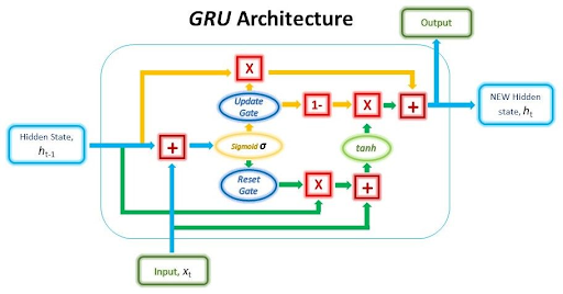
Hello! I hope you are doing great. Today, we will talk about another modern neural network named gated recurrent units. It is a type of recurrent neural network (RNN) architecture but is designed to deal with some limitations of the architecture so it is a better version of these. We know that modern neural networks are designed to deal with the current applications of real life; therefore, understanding these networks has a great scope. There is a relationship between gated recurrent units and Long Short-Term Memory (LSTM) networks, which has also been discussed before in this series. Hence, I highly recommend you read these two articles so you may have a quick understanding of the concepts. 

In this article, we will discuss the basic introduction of gated recurrent units. It is better to define it by making the relations between LSTM and RNN. After that, we will show you the sigmoid function and its example because it is used in the calculations of the architecture of the GRU. We will discuss the components of GRU and the working of these components. In the end, we will have a glance at the practical applications of GRU. Let’s move towards the first section.

What is a Gated Recurrent Unit?

The gated recurrent unit is also known as the GRU and these are the types of RNN that are designed for processes that involve sequential data. One example of such tasks is natural language processing (NLP). These are variations of long short-term memory (LSTM) networks, but they have an upgraded mechanism and are therefore designed to provide easy implementation and working features. 

The GRU was introduced in 2014 by Kyunghyun Cho, Bart van Merriënboer, Dzmitry Bahdanau, and Yoshua Bengio. They have written the paper with the title "Learning Phrase Representations using Gated Recurrent Units." This paper gained fame because it was published at the 31st International Conference on Machine Learning (ICML 2014). This mechanism was successful because it was lightweight and easy to handle. Soon, it became the most popular neural network for complex tasks. 

What is the Sigmoid Function in GRU?

The sigmoid function in neural networks is the non-linear activation function that deals with values between 0 and 1 as input. It is commonly used in recurrent networks and in the case of GRU, it is used in both components. There are different sigmoid functions and among these, the most common is the sigmoid curve or logistic curve.

Mathematically, it is denoted as: f(x) = 1 / (1 + e^(-x))

Here,

f(x)= Output of the function

x = Input value

When the x increases from -∞ to +∞, the range increases from 0 to 1.

Architecture of GRU

The basic mechanism for the GRU is simple and approaches the data in a better way. This gating mechanism selectively updates the hidden state of the network and this happens at every step. In this way, the information coming into the network and going out of it is easily controlled. There are two basic mechanisms of gating in the GRU:

  1. Update Gate (z)
  2. Reset Gate (r)

The following is a detailed description of each of them:

Update Gate (z)

The update gate controls the flow of the precious state. It shows how much information from the previous state has to be retained. Moreover, it also provides information about the update and the new information required for the best output. In this way, it has the details of the previous and current steps in the working of the GRU. It is denoted by the letter z and mathematically, the update gate is denoted as:

Here, 

W(z) =  weight matrix for the update gate

ℎ(t−1)= Previous hidden state

x(t)=  Input at time step t

σ = Sigmoid activation function

Reset Gate (r)

The resent gate determines the part of the previous hidden state that must be reset or forgotten. Moreover, it also provides information about the part of the information that must be passed to the new candidate state. It is denoted by "r,” and mathematically,

Here, 

r(t) = Reset gate at the time step

W(r) = Weight matrix for the reset gate

h(t−1) = Previous hidden state

x(t)= Input at time step

σ = Sigmoid activation function.

Once both of these are calculated, the GRU then apply the calculations for the candidate state h(t). The “h” in the symbol has a tilde at it. Mathematically, the candidate state is denoted as:

ht=tanh(Wh⋅[rt⋅ht−1,xt]+bh)

When these calculations are done, the results obtained are shown with the help of this equation:

ht=(1−zt)⋅ht−1+zth~t

These calculations are used in different ways to provide the required information to minimize the complexity of the gated recurrent unit. 

Working of Gated Recurrent Unit

The gated recurrent unit works by processing the sequential data, then capturing dependencies over time and in the end, making predictions. In some cases, it also generates the sequences. The basic purpose of this process is to address the vanishing gradient and, as a result, improve the overall modelling of long-range dependencies. The following is the basic introduction to each step performed through the gated recurrent unit functionalities:

Initialisation of GRU

In the first step, the hidden state h0 is initialized with a fixed value. Usually, this initial value is zero. This step does not involve any proper processing.

Processing in GRU

This is the main step and here, the calculations of the update gate and reset gate are carried out. This step requires a lot of time, and if everything goes well, the flow of information results in a better output than the previous one. The step-by-step calculations are important here and every output becomes the input of the next iteration. The reason behind the importance of some steps in processing is that they are used to minimize the problem of vanishing gradients. Therefore, GRU is considered better than traditional recurrent networks. 

Hidden State Update

Once the processing is done, the initial results are updated based on the results of these processes. This step involves the combination of the previous hidden state and the processed output. 

Difference Between GRU and LSTM

Since the beginning of this lecture, we have mentioned that GRU is better than LSTM. Recall that long short-term memory is a type of recurrent network that possesses a cell state to maintain information across time. This neural network is effective because it can handle long-term dependencies. Here are the key differences between LSTM and GRU:

Architecture Complexity of the Networks

The GRU has a relatively simpler architecture than the LSTM. The GRU has two gates and involves the candidate state. It is computationally less intensive than the LSTM.

On the other hand, the LSTM has three states named:

  1. Input gate
  2. Forget gate
  3. Output gate

In addition to this, it has a cell state to complete the process of calculations. This requires a complex computational mechanism.

Gate Structure of GRU and LSTM

The gate structures of both of these are different. In GRU, the update gate is responsible for the information flow from the current candidate state to the previous hidden state. In this network, the reset gate specifies the data to be forgotten from the previous hidden state. 

On the other hand, the LSTM requires the involvement of the forget gate to control the data to be retained in the cell state. The input gates are responsible for the flow of new information into the cell state. The hidden state also requires the help of an output gate to get information from the cell state. 

Training Time 

The simple structure of GRU is responsible for the shorter training time of the data. It requires fewer parameters for working and processing as compared to LSTM. A high processing mechanism and more parameters are required for the LSTM to provide the expected results. 

Performance of GRU and LSTM

The performance of these neural networks depends on different parameters and the type of task required by the users. In some cases, the GRU performs better and sometimes the LSTM is more efficient. If we compare by keeping computation time and complexity in mind, GRU has a better output than LSTM. 

Memory Maintainance

The GRU does not have any separate cell state; therefore, it does not explicitly maintain the memory for long sequences. Therefore, it is a better choice for the short-term dependencies. 

On the other hand, LSTM has a separate cell state and can maintain the long-term dependencies in a better way. This is the reason that LSTM is more suitable for such types of tasks. Hence, the memory management of these two networks is different and they are used in different types of processes for calculations.

Applications of Gated Recurrent Unit

The gated recurrent unit is a relatively newer neural network in modern networks. But, because of the easy working principle and better results, this is used extensively in different fields. Here are some simple and popular examples of the applications of GRU:

Natural Language Processing

The basic and most important example of an application is NLP. It can be used to generate, understand, and create human-like language. Here are some examples to understand this:
The GRU can effectively capture and understand the meaning of words in a sentence and is a useful tool for machine translation that can work between different languages. 

The GRU is used as a tool for text summarization. It understands the meaning of words in the text and can summarize large paragraphs and other pieces of text effectively.  

The understanding of the text makes it suitable for the question-answering sessions. It can reply like a human and produce accurate replies to queries.

Speech Recognition with GRU

The GRU does not only understand the text but is also a useful tool for understanding and working on the patterns and words of the speech. They can handle the complexities of spoken languages and are used in different fields for real-time speech recognition. The GRU is the interface between humans and machines. These can convert the voice into text that a machine can understand and work according to the instructions. 

Security measures with GRU

With the advancement of technology, different types of fraud and crimes are becoming more common than at any other time. The GRU is a useful technique to deal with such issues. Some practical examples in this regard are given below:

  • GRU is used in financial transactions to identify patterns and detect fraud and other suspicious activities to stop online fraud.
  • The networks are analyzed deeply with the help of GRU to identify malicious activities and retain the chance of any harmful process, such as a cyberattack.

Bottom Line

Today, we have learned about gated recurrent units. These are modern neural networks that have a relatively simple structure and provide better performance. These are the types of recurrent neural networks that are considered a better version of long short-term neural networks. Therefore, we have discussed the structure and processing steps in detail and in the end, we compared the GRU with the LSTM to understand the purpose of using it and to get an idea about the advantages of these neural networks. In the end, we saw practical examples where the GRU is used for better performance. I hope you like the content and if you have any questions regarding the topic, you can ask them in the comment section.

Deep Residual Learning for Image Recognition

Hey readers! Welcome to the next lecture on neural networks. We are learning about modern neural networks, and today we will see the details of residual networks. Deep learning has provided us with remarkable achievements in recent years, and residual learning is one such output. This neural network has revolutionized the design and training process of the deep neural network for image recognition. This is the reason why we will discuss the introduction and all the content regarding the changes these network has made in the field of computer vision.

In this article, we will discuss the basic introduction of residual networks. We will see the concept of residual function and understand the need for this network with the help of its background. After that, we will see the types of skip connection methods for the residual networks. Moreover, we will have a glance at the architecture of this network and in the end, we will see some points that will highlight the importance of ResNets in the field of image recognition. This is going to be a basic but important study about this network so let’s start with the first point.

What is a Residual Neural Network?

Residual networks (ResNets) were introduced by Kaiming He, Xiangyu Zhang, Shaoqing Ren, and Jian Sun in 2015. They introduced the ResNets, for the first time, in the paper with the title “Deep Residual Learning for Image Recognition”. The title was chosen because it was the IEEE Conference for Computer Vision and Pattern Recognition (CVPR) and this was the best time to introduce this type of neural network.

These networks have made their name in the field of computer vision because of their remarkable performance. Since their introduction into the market, these networks have been extensively used for processes like image classification, object detection, semantic segmentation, etc.

ResNets are a powerful tool that is extensively used to build high-performance deep learning models and is one of the best choices for fields related to images and graphs. 

What is a Residual Function?

The residual functions are used in neural networks like ResNets to perform multiple functions, such as image classification and object detection. These are easier to learn than traditional neural networks because these functions don’t have to learn features from scratch all the time, but only the residual function. This is the main reason why residual features are smaller and simpler than the other networks.

Another advantage of using residual functions for learning is that the networks become more robust to overfitting and noise. This is because the network learns to cancel out these features by using the predicted residual functions. 

These networks are popular because they are trained deeply without the vanishing gradient problem (you will learn it in just a bit). The residual networks allow smooth working because they have the ability to flow through the networks easily. Mathematically, the residual function is represented as:

Residual(x) = H(x) - x

Here,

  • H(x) = the network's approximation of the desired output considering x as input
  • x = the original input to the residual block

The background of the residual neural networks will help to understand the need for this network, so let’s discuss it.

Background for Residual Neural Network

In 2012, the CNN-based architecture called AlexNet won the ImageNet competition, and this led to the interest of many researchers to work on the network with more layers in the deep learning neural network and reduce the error rate. Soon, the scientists find that this method is suitable for a particular number of layers, and after that limit, the gradient becomes 0 or too large. This problem is called the vanishing or exploding of the gradient. As a result of this process, the training and testing errors increase with the increased number of layers. This problem can be solved with residual networks; therefore, this network is extensively used in computer vision.

Skip Connection Method in ResNets

ResNets are popular because they use a specialized mechanism to deal with problems like vanishing/exploding. This is called the skip connection method (or shortcut connections), and it is defined as:

"The skip connection is the type of connection in a neural network in which the network skips one or more layers to learn residual functions, that is, the difference between the input and output of the block."

This has made ResNets popular for complex tasks with a large number of layers. 

Types of Skip Connection in RestNets

There are two types of skip connections listed below:

  1. A short connection is a more common type of connection in residual neural networks. This allows the network to learn the residual function at a rapid rate. In residual learning, these are used in the adjacent residual blocks. In this way, the network learns about the residual function within the block. An example of a short connection is that the residual block learns to add a small amount of noise to the input or can change the contrast of the input image through this.
  2. The long skip connection connects the input of the residual block to the output of the much later layer of the network. This network cannot work on a small scale but can add a small amount of noise to the entire image or change the contrast of the whole image. Thai allows the network to learn the long-range dependencies.

Both of these types are responsible for the accurate performance of the residual neural networks. Out of both of these, short skip connections are more common because they are easy to implement and provide better performance. 

Architecture of Residual Networks

The architecture of these networks is inspired by the VGG-19 and then the shortcut connection is added to the architecture to get the 34-layer plain network. These short connections make the architecture a “residual network” and it results in a better output with a great processing speed.

Deep Residual Learning for Image Recognition

There are some other uses of residual learning, but mostly these are used for image recognition and related tasks. In addition to the skip connection, there are multiple other ways in which this network provides the best functionality in image recognition. Here are these:

Residual Block

It is the fundamental building block of ResNets and plays a vital role in the functionality of a network. These blocks consist of two parts:

  1. Identity path
  2. Residual path

Here, the identity path does not involve any major processing, and it only passes the input data directly through the block. Whereas, the network learns to capture the difference between the input data and the desired output of the network. 

Learning Residual

The residual neural network learns by comparing the residuals. It compares the output of the residual with the desired output and focuses on the additional information required to get the final output. This is one of the best ways to learn because, with every iteration, the results become more likely to be the targeted output.

Easy Training Method

The ResNets are easy to train, and the users can have the desired output in less time. The skip connection feature allows it to go directly through the network. This is applicable even in deep architecture, and the gradient can flow easily through the network. This feature helps to solve the vanishing gradient problem and allows the network to train hundreds of layers efficiently. This feature of training the deep architecture makes it popular among complex tasks such as image recognition. 

Frequent Upadation of Weight

The residual network can adjust the parameters of the residual and identity paths. In this way, it learns to update the weights to minimize the difference between the output of the network and the desired outputs. The network is able to learn the residuals that must be added to the input to get the desired output.

In addition to all these, features like performance gain and best architecture depth allow the residual network to provide significantly better output, even for image recognition. 

Conclusion

Hence, today we learned about a modern neural network named residual networks. We saw how these are important networks in deep learning. We saw the basic workings and terms used in the residual network and tried to understand how these provide accurate output for complex tasks such as image recognition.

The ResNets were introduced in 2015 at a conference of the IEE on computer vision and pattern recognition (CVPR), and they had great success and people started working on them because of the efficient results. It uses the feature of skip connections, which helps with the deep processing of every layer. Moreover, features like residual block, learning residuals, easy training methods, frequent updates of weights, and deep architecture of this network allow it to have significantly better results as compared to traditional neural networks. I hope you got the basic information about the topic. If you want to know more, you can ask in the comment section.

Transformer Neutral Network in Deep Learning

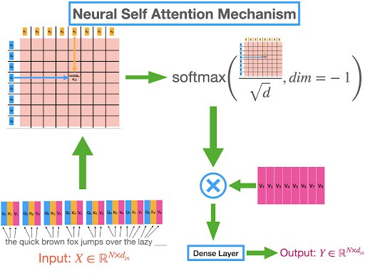
Deep learning is an important subfield of artificial intelligence and we have been working on the modern neural network in our previous tutorials. Today, we are learning the transformer architecture neural network in deep learning. These neural networks have been gaining popularity because they have been used in multiple fields of artificial intelligence and related applications.

In this article, we will discuss the basic introduction of TNNs and will learn about the encoder and decoders in the structure of TNNs. After that, we will see some important features and applications of this neural network. So let’s get started.

What are Transformer Neural Networks

Transformer neural networks (TNNs) were first introduced in 2017. Vaswani et al. have presented this neural network in a paper titled “Attention Is All You Need”. This is one of the latest additions to the modern neural network but since its introduction, it has been one of the most trending topics in the field of neural networks. The basic introduction to this network:

"The Transformer neural networks (TNNs) are modern neural networks that solve the sequence-to-sequence task and can easily handle the long-range dependencies."

It is a state-of-the-art technique in natural language processing. These are based on self-attention mechanisms that deal with the long-range dependencies in sequence data. 

Working Mechanism of RNN

As mentioned before, the RNNs are the sequence-to-sequence models. It means these are associated with two main components:

  1. Encoder
  2. Decoder

These components play a vital role in all the neural networks that deal with machine translation and natural language processing (NLP). Another example of a neural network that uses encoders and decoders for its workings is recurrent neural networks (RNNs).

RNN Encoder’s Working

The basic working of the encoder can be divided into three phases given next:

Input Processing

The encoder takes the input in the form of any sequence such as the words and then processes it to make it useable by the neural network. Thai sequence is then transformed into the data with a fixed length according to the requirement of the network. This step includes procedures such as positional encoding and other pre-processing procedures. Now the data is ready for representation learning. 

Representation Learning

This is the main task of an encoder. In this, the encoder captures the information and patterns from the data inserted into it. It takes the help of recurrent neural networks RNNs for this. The main purpose of this step is to understand dependencies and interconnected relationships among the information of the data. 

Contextual Information

In this step, the encoder creates context or hidden space to summarise the information of the sequence. This will help the decoder to produce the required results. 

RNN Decoder’s Working

Source text

The decoder takes the results of the contextual information from the encoder. The data is in the hidden state and in machine translation, this step is important to get the source text. 

Output Generation

The decoder uses the information given to it and generates the output sequence. In each step of this sequence, it has produced a token (word or subword) and combined the data with its own hidden state. This process is carried out for the whole sequence and as a result, the decoded output is obtained.

The transformer pays attention to only the relevant part of the sequence by using the attention mechanism in the decoders. As a result, these provide the most relevant and accurate information based on the input.

In short, the encoder takes the input data and processes it into a string of data with the same length. It is important because it adds contextual information to the data to make it safe. When this data is passed to decoders, the decider has information on the contextual data, and it can easily decode the information and pay attention to the relevant part only. This type of mechanism is important in neural networks such as RNNs and transformer neural networks; therefore, these are known as sequence-to-sequence networks.

Features of Transformer Neural Network Architecture

The TNNs create the latest mechanism, and their work is a mixture of some important neural networks. Here are some basic features of the transformer neural network:

Self Attention Mechanism

The TNNs use the self-attention mechanism, which means each element in the input sequence is important for all other elements of the sequence. This is true for all the elements; therefore, the neural network can learn long-range dependencies. This type of mechanism is important for tasks such as machine translation and text summarization. For instance, when a sentence of different words is added to the TNNs, it focuses more on the main word and applies the calculations to make sure the right output is performed. When the network has to translate the sentence “I am eating”, from English to Chinese, it focuses more on “eating” and then translates the whole sentence to provide the accurate result.

Parallel Processing

The transformer neural networks process the input sequence in a parallel manner. This makes them highly efficient for tasks such as capturing dependencies across distant elements. In this way, the TNNs takes less time even for the processing of large amount of data.  The workload is divided into different core processors or cores. The advantage of multiple machines in this network makes them scalable. 

Multi-head Attention

The TNNs have a multi-head mechanism that allows them to work on the different sequences of the data simultaneously. These heads are responsible for collecting the data from the pattern in different ways and showing the relationship between these patterns. This helps to collect the data with great versatility and it makes the network more powerful. In the end, the results are compared and accurate output is provided.

Pre-trained Model

The transformer neural networks are pre-trained on a large scale. After this process, these are fine-tuned for particular tasks such as machine translation and text summarization. This happens when the usage of labeled data is on a small scale in the transformer. These networks learn through this small database and get information about patterns and relationships among these datasets. These processes of pre-training and fine-tuning are extremely useful for the various tasks of natural language processing (NLP). Bidirectional Encoder Representations from Transformers (BERT) is a prominent example of a transformer pre-trained model.

Real-life Applications of TNNs

Transformers are used in multiple applications and some of these are briefly described here to explain the concept:

  • As mentioned before, machine translation is the basic application of a transformer neural network. Different platforms are using this for the translation of one language into another at different levels. For instance, Google Translate uses the transform to translate the content over more than 100 languages.
  • Text summarization is another important application of TNNs. This neural network can read long articles in just a bit and can provide a summary without skipping any important concept.

  • The question answering is easy with the transformer neural network. The text is inserted into the QA application and it provides instant replies and answers. The text may be on any topic therefore, such software is used in almost every field of life.
  • The TNNs are widely used to create software that can instantly provide the codes for different problems and applications. A good example in this regard is the AlphaCode software which is used for the generation of code with the help of simple prompts. This is generated by DeepMind and the TNNs are used for the basic working of this software.
  • The chatbots and websites are being created with the TNNs that can easily provide creative writing on different topics. For instance, the Chat-GPT is a large language model that is created by openAI. It can create, edit, and explain different text types such as poems, scripts, codes, etc.
  • The automatic conversation is an important application of TNNs because it has omitted the need for physical operators on different systems. The chatbots and conversational AI systems can now talk to the customers and users and provide them the logical and human-like replies in no time.

Hence, we have discussed the transformer neural network in detail. We started with the basic definition of the TNNs and then moved towards some basic working mechanisms of the transformer. After that, we saw the features of the transformer neural network in detail. In the end, we have seen some important applications that we use in real life and these use TNNs for their workings. I hope you have understood the basics of transfer neural networks, but still, if you have any questions, you can ask in the comment section.

Introduction to Generative Adversarial Networks

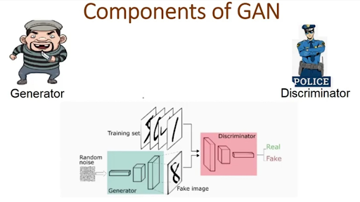
Deep learning has applications in multiple industries, and this has made it an important and attractive topic for researchers. The interest of researchers has resulted in multiple types of neural networks we have been discussing in this series so far. Today, we are talking about generative advertising neural networks (GAN). This algorithm performs the unsupervised learning task and is used in different fields of life such as education, medicine, computer vision, natural language processing (NLP), etc. 

In this article, we will discuss the basic introduction of GAN and will see the working mechanism of this neural network, After that, we will see some important applications of GANs and discuss some real-life examples to understand the concept. So let’s move towards the introduction of GANs.

What are Generative Adversarial Networks?

Generative Adversarial Networks (GANs) were introduced by Ian J. Goodfellow and co-authors in 2014. This neural network gained fame instantly because it provided the best performance on its own without any external supervision. GAN is designed to take the data in the form of text, images, or other structured data and then create the new data by working more on it. It is a powerful tool to generate synthetic data, even in the form of music, and this has made it popular in different fields. Here are some examples to explain the workings of GANs:

  • GANs are used to generate photorealistic images of people that do not exist in real life, but these can be generated by using the data provided to them.
  • GANs can create fake videos in which people are saying words and doing tasks that are not recorded by the camera but are generated artificially with the GANs.
  • People can use GANs to create advanced and better products and services by providing data on present products and services.
  • We will discuss the applications of GANs in detail in just a bit.

GAN Architecture

The generative advertiser networks are not a single neural network, but their working structure is divided into two basic networks listed below:

  1. Generator
  2. Discriminator

Collectively, both of these are responsible for the accurate and exceptional working mechanism of this neural work. Here is how these work:

Working of GANs

The GANs are designed to train the generator and discriminators alternatively and to “outwit” each other. Here are the basic working mechanisms:

Generator

As the name suggests, the generators are responsible for the creation of fake data from the information given to them. These networks take the noise from the data and, after studying it, create fake data. The generator is trained to create realistic and related data to minimize the ability of the discriminator to distinguish between real and fake data. The generator is trained to minimize the loss function:

L_G = E_x[log D(x)] + E_z[log (1 - D(G(z)))]

Here,

  • x = real data sample
  • z = random noise vector
  • G(z) = generated sample
  • D(x) = probability that the discriminator outputs that x is real

Discriminator

On the other hand, the duty of the discriminator is to study the data created by a generator in detail and to distinguish between different types of data. It is designed to provide a thorough study and, at the end of every iteration, provide a report where it has identified the difference between real and artificial data.

The discriminator is supposed to minimize the loss function:

L_D = E_x[log D(x)] + E_z[log (1 - D(G(z)))]

Here, the parameters are the same as given above in the generator section.

This process continues, and the generator keeps creating data and the discriminator keeps distinguishing between real and fake data until the results are so accurate that the discriminator is not able to make any difference. These two are trained to outwit each other and to provide better output in every iteration.

Generative Adversarial Network Applications

The application of GANs is similar to that of other networks, but the difference is, that GANs can generate fake data so real that it becomes difficult to distinguish the difference. Here are some common examples of GAN applications:

GAN Image Generation

GANs can generate images of objects, places, and humans that do not exist in the real world. These use machine learning models to generate the images. GANs can create new datasets of image classification and create artistic image masterpieces. Moreover, it can be used to regenerate the blur images into more realistic and clear ones.

Text Generation with GANs

GAN has the training to provide the text with the given data. Hence, a simple text is used as data in GANs, and it can create poems, chat, code, articles, and much more from it. In this way, it can be used in chatbots and other such applications where the text is related to the existing data. 

Style Transfer with GANs

GANs can copy and recreate the style of an object. It studies the data provided to it, and then, based on the attributes of the data, such as the style, type, colours, etc., it creates the new data. For instance, the images are inserted into GAN, and it can create artistic works related to that image. Moreover, it can recreate the videos by following the same style but with a different scene. GANs have been used to create new video editing tools and to provide special effects for movies, video games, and other such applications. It can also create 3D models. 

GANs Audio Generation

The GANs can read and understand the audio patterns and can create new audio. For instance, musicians use GANs to generate new music or refine the previous ones. In this way, better, more effective, and latest audio and music can be generated. Moreover, it is used to create content in the voice of a human who has never said those words generated by GAN.

Text to Image Synthesis

The GAN not only generates the images from the reference images, but it can also read the text and create the images accordingly. The user simply has to provide the prompt in the form of text, and it generates the results by following the scenario. This has brought a revolution in all fields.

Hence, GANs are modern neural networks that use two types of networks in their structure: generators and discriminators to create accurate results. These networks are used to create images, audio, text, style, etc that do not exist in the real world but these can create new ones by reading the data provided to them. As the technology is moving towards advancements, better outputs are seen in the GANs' performance. I hope you have liked the content. You can ask anything related to the topic in the comment section.

Syed Zain Nasir

I am Syed Zain Nasir, the founder of <a href=https://www.TheEngineeringProjects.com/>The Engineering Projects</a> (TEP). I am a programmer since 2009 before that I just search things, make small projects and now I am sharing my knowledge through this platform.I also work as a freelancer and did many projects related to programming and electrical circuitry. <a href=https://plus.google.com/+SyedZainNasir/>My Google Profile+</a>

Share
Published by
Syed Zain Nasir