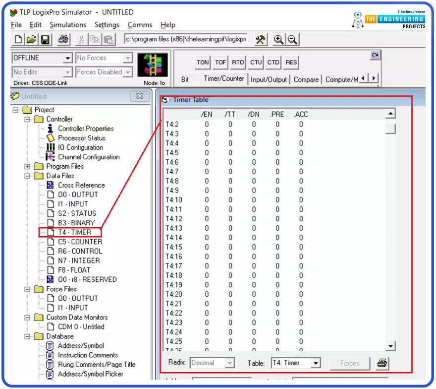
Advance Timer Functions in PLC Ladder Logic Programming

Believing in the essence of timers in ladder logic programming, we come today with a new tutorial in which we are going to show you all about timers, the types of timers, what’s inside timers’ block of parameters, variables, and bits. In addition, techniques for using timers will be explored, and for sure, we are going to practice what we learn using the simulator. So let’s get started with our tutorial.

Timers in ladder logic programming

Guys, this is not the first time we’ve talked about timers. However, this time we are going to look into timers deeply and use the glasses of practical approach. So figure 1 shows the most important types of timers in ladder logic from left to right: the on-delay, off-delay, and retentive timers. There are differences in functionality. However, they all have the same parameters, variables, and bits. For example, the on-delay timer (TON) works by starting counting by getting the high logic state of its input. And bit goes ON when and only when the counter reaches the preset value. While the off-delay timer (OFF-DELAY) employs starting with the high logic of its Done bit once it has a high logic of its input. And when its high input stat is gone and turns to low. It starts counting until reaching the preset value, and then the done bit goes off. On the other hand, the retentive timer keeps accumulating the time while the input is energized until it reaches the preset value, at then the Done bit goes on. You can see, my friends, how are different in functionality to help you get a way for every problem related to timers. Despite that variety in behavior, they have the same data, as you can see in each timer block. So now, what are these data, and how can we utilize them in ladder logic programming? that is what we are going to learn together in this tutorial.

Timer data in PLC

Well! Timer data can be demonstrated in figure 2. You can see guys in the tree view windows below; the data section shows the timers data in which there are dozens of timers you can use through long your program. But what does the data include? Well! The data has timer bits and variables, as shown on the right side of the window. The most important variables are the preset variable (PRE), in which we set the value of the time at which we require the timer to act ON. The other variable is the accumulator variable ACC that we use to know what the counted time is so far. The logic says the timer keeps increments accumulator until reaching the preset value. Okay, then what happens when the accumulator reaches the preset value? Exactly, the timer needs to indicate that he reaches the target.  There are so-called timer bits like the timing bit TT that reports the timer is timing, and the DONE bit that tells the accumulator has reached the preset value. And also the EN bit that shows the completion of execution of the timing instruction.

Most Common PLC Timer Types

Well, timers can be categorized based on their functionality and the way they work. For instance, the ON-DELAY timer starts timing when it gets a trigger signal which is the high state of its input. By reaching the preset value, the output will have been energized as long as the input is high. Please, guys, see the timing diagram in Figure 3 which depicts the timing diagram of the input and output of the ON-DELAY timer. It shows the timer contact goes on after counting the preset time value since it receives a high logic on its input coil.

The second but same important kind of timer is the OFF-DELAY timer. This timer starts energizing its contact or output from the moment it receives high logic input. Then after that input goes low, the output remains high in the logic state for as long as the preset value has been specified. Please, my friends, find the operation cleared in figure 4 below, which demonstrates the operation by the language of the time. In this example, the timer coil has been energized, and its contact goes high. And when the coil de-energized, the contact remained high for 5 seconds which is the preset amount of time of the timer.

The third timer we are going to show today is the retentive timer. So what does that timer do? Well, that timer accumulates the time whenever its coil is ON. The timing diagram is shown below in figure 5.  More details about the timing diagram of retentive timers, what figure 5 demonstrates. You can notice, my friends, as long as the input is high, the timer accumulator keeps accumulating the time until one reset signal appears, then it resets the time. But it returns back, accumulating the time whenever the input is true.

Now we will show some examples to let you understand how to employ the timer variables and bits as well. Figure 6 shows the timer block of an OFF-DELAY timer. You can see, guys, the timer’s name is T4:1, the time base is set to 00.1, and the preset value is set to 100, meaning it is designed to time for 10 seconds that can be determined by multiplying the time base to the preset value. Also, you can see that the first rung used input I:1/0 to enable the timer by energizing its coil. Rungs 1 to 3 show how you guys might use the timer bits. For example, in rung number 1, the enable bit of the timer is used to energize output O:2/0. Similarly, the timing bit TT of the timer is utilized to turn on output O:2/1 in rung 002. While the done bit DN energizes output O:2/2 as in rung 003.

Simulating one example

Here it is the simulation of one example to show how the timers bits and variables can set and used. In figure 7, the timer of type on-delay T4:4 is used and set to time for 10 seconds by setting the preset to 100 and the time base to one-tenth 0.1. the timer’s bits are used as you can see my friends to activate different outputs.

Example showing timers types

Another example demonstrated in figure 8 to show the on-delay and off-delay timers working together to fulfill the requested logic.

Retentive Timer example in Ladder Logic

Figure 10 shows an example to demonstrate the utilization of a retentive timer type. You can see the timer block of the retentive timer RTO and how it is accumulating the time whenever the input is high without resetting when the input is turned off.

Timers programming techniques

Going to one of the most important parts of our tutorial is how professionally you guys can use the timers to solve whatever problem you have. The techniques to use timers that come with experience. For example, figure 11 shows the cascading timing technique in which you can use multiple timers based on each other in a cascading way. You see, guys, how timer T4:2 depends on the Done bit of timer T4:1 in cascading approach. Why do we need to use two timers in such a way when we can use only one with a preset value equal to the sum of the two timers? That’s smart to be asked. But the answer also is intelligent, which tells us we might need to do some action in between. For example, when timer number one has done timing, we might energize one output, and after the second, we perform another action depending on the first timer.

Reset the timers in Ladder Logic

Figure 12 shows the technique to reset the timer by having one normal close contact in the way of its input to control energizing the timer coil. In that very example demonstrated by figure 12, the timer Done bit itself is used to reset the timer, meaning that when the time contact acted ON, it is the time to reset the timer and like that, we can guarantee the timer keeps repeating the process forever.

And at that point, I would like to thank all my friends for following me till the end of that tutorial, and I hope you have learnt some knowledge and enjoyed practicing one of the most important topics in ladder logic programming, Timers. For recapping have nailed the timers by demonstrating the variables and bits of the timers and the types and techniques of using the timers to flexibly and professionally can deal with different situations and solve any problems related to using the time.

Traffic Signal Control with PLC Ladder Logic Programming

The traffic light is one of the most important applications we see everyday everywhere we go back and forth. Controlling traffic signs was managed by people which was very problematic and headache on travelers and the officers as well. But nowadays, most traffic lights are controlled by automatic control systems. The brain that handles the complicated logic behind the traffic light control system is a PLC and one programmer like you guys has written its logic. So today we have come back to enjoy programming such a critical and large project by using ladder logic programming and for sure will apply the code and the logic we write into the simulator to check its correctness.  

Problem we try to solve

First of all, the scene we captured below by figure 1 shows two ways to cross a traffic signal, the biggest and most complicated traffic sign you might see anywhere you go. We need to go through the logic and requirements and then list these alongside with the restrictions for realizing the safety which is very critical and crucial right here for saving people and vehicles traveling in each way in  the cross traffic light. The complete project will be divided into two tasks to simplify the project and each task will be an exercise for you guys to do. So without any further delay let’s jump into our project’s exercises.

Project description

As you can see in figure 2, there are two faces of three traffic lights, one for each side way to control the cross traffic light. Each traffic light side has three indicators RED, green, and Ampere to represent the stop, ready-to-cross, and about-to-change that tells the car drivers and pedestrians when to stop and what time they can continue crossing. Each lamp has assigned to one output as you can see guys in the image. Our task is to control the timing of lighting each indicator to achieve the whole process. As we have mentioned earlier we are going to work the project into couple of milestones. So let we names two milestones in the first one we are going to control one way and will complement the work by adding the code to manage the two crossways by reaching that point we will have completed our mission. So let’s getting into the work.

The one way control Part 1

Table 1 below lists the required amount of time and the sequence of the lighting of each indicator for controlling one way of the cross traffic light control project. As listed in the table below, the red light is connected to output O:2/00 and it is required to light it for 12 seconds. Then the green light that is connected to output O:2/02 should be lit for 8 seconds and finally the Amber light for 4 seconds which is connected to output O:2/01. Remember my friends, we need to repeat the process forever.

RED

GREEN

AMBER

12 Sec.

8 Sec.

4 Sec

The ladder logic code 

Figure 3 shows the program of the first part to control one way. You notice guys the program is mainly based on utilizing timers. The idea is simply to start with an on-delay timer of the whole period which is 24 seconds. As it is clear the first rung energizes the timer T4: 0 to start timing for 24 seconds. Then by comparing the accumulating time, the second rung activate the green light for 8 seconds by using the comparing instruction LES in the way like keep energize the red light that connected to O:2/0 as long as the the accumulator of T4:0 which is is T4:0.acc less than 12 seconds. In the same way, in the period between 12 to 20 seconds the green light is activated for 8 seconds thanks to using the comparing instructions GRT and LES. And finally command the amper light to energize after 4 sec to the end. Notice my friend to let the process repeat forever, the timer is cleared or restarted by enabling the flag B3:1/0. Let us test the logic we have just implemented to see if it can work fulfilling the requirements or not.

Testing part 1 using simulator

The evaluation of the first part is depicted by figure 4. See guys the red sign is lit for 12 seconds and the green light follows for 8 seconds as shown in figure 5.

And figure 6 below depicts the ampere lighting for 4 seconds. Now you can see we have completed the first part.

But wait my friends as we can not proceed with the project and let it be working at this stage do you know why? Exactly, it is not safe because the control has not been programmed for the other way so the results would be sad as shown in figure 7.

The project second part

As we mentioned earlier, the project has been achieved by dividing it into two parts. In the first part that we have just demonstrated above including the ladder logic program and testing using our simulator. That very part, part one can control one way traffic but we have two running traffic lights that should be considered. From here we are going to show the second part of the project. Let us start with the requirements.

Part two the requirements

Table 2 below asks you guys to control both traffic ways to have the red light on one side for a 12 seconds period time in which you need to allow the green light of the other way to light for 8 seconds and then the Amber light will be permitted for the next 4 seconds. The same logic will be applied on the reverse side. On another word, side number one is red with green and amper of side number two. Also, red of side number two with green and amper of side number one. Let us see the ladder logic and description of the implemented logic in the following section.

Red = O:2/00

Green = O:2/02

Amber = O:2/01

Green = O:2/06

Amber = O:2/05

Red = O:2/04

8 Sec.

4 Sec.

8 Sec.

4 Sec.

Logic of the second part

For the length of the program” We have divided it into two pieces. The first one is shown in the figure 8. You can see guys, it is similar to utilize the timers and compare instructions to accomplish the project. Like part one but adding amendments to combine the second part requirements. in the third rung you notice my friends we have added just restriction to not letting the green and amber light of one side while the green or amber does in the other side and vise versa. So what we are doing in the first four rungs is to handle one way traffic signal with restricting the other side when it is needed. Now let us move to the second part of code.

Figure 9 demonstrates the control of the other side by adding the logic for the green of the other side as in rung 5 considering the restriction of the green and amber of the side one at that time. Then in rung 7, the control for the amber light of side 2 considers inhibiting the amber and green of the side one for avoiding the crash to happen. And at last the red light is energized for 12 seconds in which the green and amber of the other side are not prohibited. Now time to test our logic has come so let us go testing that program.

Testing the completed project

Here you can see friends the test of the completed project in figure 10. Notice that one side has the green light on and the other side shows the red is lighted. As a result, the side with green light on allows the vehicles to pass while the side with red sign lighted in bit cars from passing.

More testing to check the opposite scenario for checking the cross traffic logic. Figure 11 shows the other side amber sign is on while the red of the opposite side is on. Therefore, the cars are allowed with the side that has the amber light on. On the other hand, the side that has the red light is one prevent cars from passing.

My friends, I really appreciate you following up to that very point and hoping you have got to learn and enjoy practicing one of the most important projects that you might see in everywhere you go in your daily life. Please know one thing which is very important that, the code we have implemented just right here is not the only way to solve such project. There are dozens of way to code such a project so please try your way without hesitation and keep trying to increase your knowledge and boost professionally in ladder logic programming.  Thanks again guys and let us meet in another tutorial and project of the real life problem to learn and enjoy practicing ladder logic programming together.

Automatic Garage Door with PLC Ladder Logic

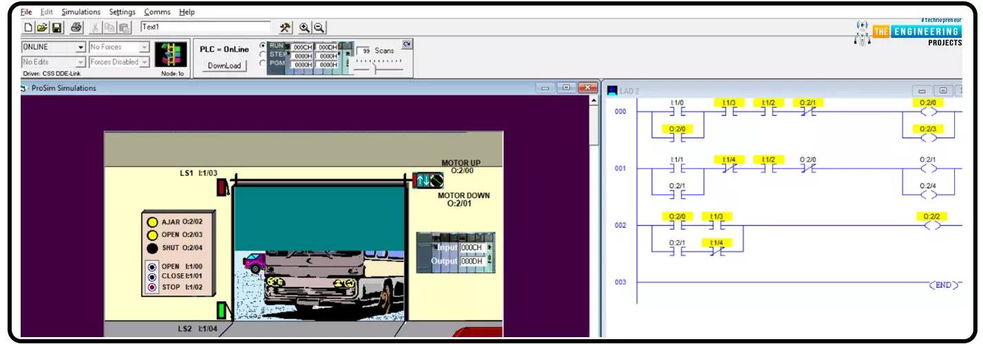
Hello my friends! I hope your doing very good. Today we are going to practice what we have learnt through the ladder logic tutorial series. We bring a new .project which is mostly exist in our daily life that is electrical door control. in garage for domestic and public garage, you should found automatic garage gate or door that is controlled by the PLC ladder logic program. So today we are going to implement the project including determining the input and output components, design the logic, programming and testing using the simulator.

Project details

Figure 1 shows the project’s components, inputs and outputs that are included in controlling the garage door. As you can see my friends, there are inputs like open, close, and stop requested by push buttons. Also, you can see sensors like the two limit switches on the bottom and on the top to prevent overload that might have occurred on the motors. Moving to the outputs, there are motor up and down directions, open, close, and ajar status indicators lamps. So what is the next step in our plan to achieve such job? Of course we need to list these inputs and outputs and give them addresses. Then we design the logic based on the user requirements and the safe operation.

Inputs and Outputs list

Table 1 lists the inputs and outputs showing the name in the first column, the description In the second column, while the addresses are listed in the last column.


Component 

Description 

Address00

Open push button

One of the inputs to request open operation  

I: 1 / 00

Close push button

One of the inputs that enables user to shut down the door

I: 1 / 01

Stop push button

The push button to stop operation at any time

I: 1 / 02

Limit switch 1

A sensor to stop opening operation beyond the opening limits

I : 1 / 03

Limit switch 2

A sensor to stop closing operation beyond the closing limits

I : 1 / 04

Shut down indicator  

One of the outputs that tells the shutdown operation is in progress using an Indicator lamp 

O: 2 / 04

Open door indicator

One of the outputs that tells the opening door operation is in progress using an Indicator lamp 

O: 2 / 03

Ajar door status

One of the outputs that tells the door is ajar using an Indicator lamp 

O: 2 / 02

Motor Up

A relay that directs the door in opening direction 

O: 2 / 00

Motor Down

A relay that directs the door in closing direction 

O: 2 / 01

The logic operation

After receiving the requirements of the client that tell how the door will be operated, managed, and controlled, we need to add the restrictions and safety conditions that secure the equipment like the motor, supply, sensing components. So the following lines state the operation and restrictions that need to be followed to achieve the designated task as follows:

  • The door opening and or closing shall be stopped at any time user / operator hit stop push button

  • The door shall open by requesting opening operation using the designated push button

  • The door shall close by requesting shut down operation using the designated push button

  • The indicator lamp of opening operation shall be lit while opening operation is in progress

  • The indicator lamp of closing operation shall be lit while shut down operation is in progress

  • The ajar status lamp shall be lit at any time the door is not fully opened or totally closed

Restrictions:

  • The opening operation can not be requested while shut down process is in progress

  • The shut down operation can not be requested while opening operation is in progress

  • The opening operation can not proceed any further beyond the designated limit to avoid any overload on the motor

  • The shut down operation can not proceed any further beyond the designated limit to avoid any overload on the motor.

Ladder Logic Code for Garage Door Project

The ladder logic program of the project is shown by figure 2. It shows two rungs, one for opening process and second for the shut down operation. The program can be more lengthy but we professionally resumed it in only two main rungs. The first rung represents the door opening operation in which, open push button initiates the opening process and the latching is there to let the opening process continue till the limit switch LS1 contacted or the stop is requested by hitting the stop push button. In addition, security of the process has been considered by including the condition of not having a shutdown process in progress represented by O:2/1. On the other hand, the shut down process is represented by the second rung. The shut down process initiated by the shut down push button and latching the door closing relay for continuing the shut down process unless one of the restriction conditions is met. The restriction conditions of shut down are the limit switch LS2, the door opening in progress, or a stop has been requested by operator using the stop push button. Also, indicator of the process status are included to show the opening operation thanks to the door opening indicator and the shutdown indicator. But we missed the ajar status of the door so let us add one rung for that.

As you see guys, the third rung has been added to implement the ajar status. It is simply clear that when the opening is in progress without reaching to the fully open indicator, or the shut down process is in progress without reaching to the totally closed, the ajar lamp is energized. Now let us go testing what we have coded so far and see if it is correct or not. But first you guys should sit and list the test cases that you should try to make sure the system is going to perform correctly and safely as well.

Testing the project

Door Opening test

In this test , we hit the opening door push button to request opening the door. As you see my friends, the door is opening as in figure 3 and the opening indicator is lit. also you can see the ajar indicator is lighted because the door is not reached the final opening position.

Figure 5 shows the state of the process after reaching the final position for opening the door. It is clear the process safely completed and the limit switch LS1 is gone green. Also the ajar status and opening indicators have been turned off.

Door closing test

In this test , we hit the door shut down push button to request closing the door. As you see my friends, the door is closing as in figure 6 and the closing indicator is lit. also you can see the ajar indicator is lighted because the door has not reached the final shut down position.

Figure 7 shows the state of the process after reaching to the final position for closing the door. It is clear the process safely completed and the limit switch LS2 is gone red. Also the ajar status and shut down indicators have been turned off.

Security and Safety Test

In this test case we want to request opening .the door while it is shuting down and try to request shut down the door while it is opening to see is there any issue or not. Figure 8 shows what is going on when we requested opening the door while a shuting down process is inprogress. You can see guys in rung number one, the opening push button ,is pressed as circled and highlighted see I:1/0. However, the requested process has not performed due to the restriction that the shutdown process should not be in progress. Same thing when opening door is in progress, shut down requests are forbidden.

Control Project with Ladder Logic Programming

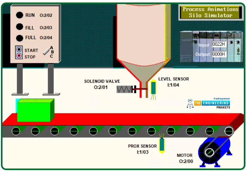
Hey guys! hope you are all very well. Today I come to you with a new process to learn, program, and simulate for practicing ladder logic more and more. The process we are going to implement today is a very common process that could be there in many many industries which is a silo process that aims to automate the process of filling containers or bottles with a liquid. Figure 1 shows the complete scene of the process including the system components, switches, indicators, sensors, and actuators that are integrated to make the system operate. Briefly and before going into deep details, let’s state what the system does and how it operates. Well! The system automatically fills the boxes that are traveling on the conveyor which is driven by a motor. They are filled with a liquid stored in the silo shown in the middle of figure 1. The process operates continuously from the moment we hit the start button shown in the tail of the control panel on the left side of figure 1 until termination of the process is requested by pressing the stop push in the same panel. Many inputs and outputs are utilized to address the sensors, switches, push buttons, motors, and valves. So let’s get started on the project.

Project Logic Philosophy

As we have thought, the first step in the development of a control system is to sit with the operator or the client to get to comprehend how the system works including all details and scenarios. So the system starts by receiving the kickoff by hitting the start pushbutton. Unless there is no stop has been requested or faults, the box moves on the conveyor that is driven by a motor until it reaches the filling station which is at the silo. At that position, the box should stop for filling, and the flow of the liquid starts and goes on until the box is full. Then, it is time for the box to continue its journey to the end of the conveyor and another box commences a new trip for filling. At any time a stop is requested, the system should halt until a command to continue is presented. Operation status should be shown thanks to indicators showing the run, fill, and full status. Now, friends, that’s all the story we have gotten by sitting with the client or the operator who requested us to implement his system. have understood the requested silo operation? Well done! I know it is simple to understand but what is the next step? Yes, the next station in the project is to interpret the story narrated by our client into operation sequences and conditions and determine the list of inputs and outputs to get that project done. 

Logic sequence

The aims of the project we are going to implement is to implement the ladder logic program that execute the narrated logic of SILO by client. The logic can be resumed in the following sequence of operations: 

  • The batch process can be started or stopped at any point of execution 

  • Indicator lamps should be appropriately controlled to present the run, fill, and full statuses of the operation throughout the whole process.

  • All actuators should be stopped at any time a termination requested by the end user

  • The FULL lamp is switched on showing the full status of the box as long as the box at its filling position under the silo.

  • After converting the logic narrative received from the client into clear logic sequences, now the time comes to list the inputs and outputs to use to accomplish these logic sequences. In the next section, the complete list of inputs represented by sensors and switches and outputs represented by motors, valves, and light indicators. 

Project I/Os

Figure 2 shows the location and address of all inputs and outputs used in this project. Also, the table below lists all inputs and outputs of the project including descriptions and addresses. The control panel on the lift shows two inputs that enable an operator to start and stop the operation. Also, it shows indicators showing the status of the operation throughout the whole process. These status indicators are RUN. FILL, FULL to show the process is running, the box is filling, and when it is full. Also, it shows the motor that drives the conveyor and the proxy sensor that detects the position where the box is exactly under the silo and ready to be filled for initiating the filling process. Also, a level sensor is utilized to determine when the box is filled up to full. In addition, a valve is used to open and close the silo.

  Table 1: list of inputs and outputs of the project     

IO

type

Description

Address

RUN

Output

Indicator lamp to show the running status

Q2.2 for siemens

O:2/02 for AB

FILL

Output

An indicator lamp to show the filling process is in progress

Q2.3 for siemens

O:2/03 for AB

Full 

output

An indicator lamp to show the full status of the box

Q2.4 for siemens

O:2/04 for AB

MOTOR

Output 

The main motor drives the conveyor to take the boxes through their journey  

Q2.0 for siemens

O:2/00

Valve

Output

A solenoid valve to control the silo to open or close according to the logic

Q2.1 for siemens

O:2/01 for AB

Start

input

A pushbutton enables the operator to start the process

I1.0 for siemens

I:1/00 for AB

Stop 

Input 

A pushbutton enables the operator to stop the process

I1.1 for siemens

I:1/01 for AB

Level sensor

input

A level switch to detect the level of the liquid being filled into the box

I1.4 for siemens

I:1/04 

Proximity switch

Input 

A proximity switch to sense the position of the approaching box 

I1.3 for siemens

I:1/03 


Logic Flow Diagram

Guys, this is not an essential step to accomplish the project development. But this is one of the professional ways to represent graphically the design of the logic. Figure 3 depicts the logic of the silo project graphically. You can follow paths of logic to understand how we can chart the logic flow running in our head graphically to help in writing the correct and precise code. For example, to run the conveyor motor, the start button is pressed and checked if a stop is requested, if not the run lamp indicator will be energized and latched as long as no stop is requested. Then check if a fill process is in progress. If not then the motor of the conveyor will keep running. But the question is how to know if the fill is in progress or not. On the left side of the chart, you can see if the proxy switch is on and the level switch does not show full, then the filling process is in progress. Also, if the level switch shows not full then the valve will keep open to continue filling the boxes.

Ladder Logic Programming of the project

Now we have just arrived at what you are waiting for! I know you want to practice programming and then simulation. Figure 4 shows the program of the silo project while the left part shows the initial state of our simulation. The first rung is to energize the run indicator when the start pushbutton is hit and no stop is requested noting the latch as we have learned. In the second rung, knowing the run is the status of the operation and no filling process is in progress, then the motor is running. In the third rung, the filling status can be determined by the proximity switch showing the boss is at the position were ready to fill and full status is not there. While the full status can be determined in the last rung when the level switch is on showing level has reached the full limit of the box and pursuing the proximity switch tells the box is on the filling spot. Before that very last rung, the valve of the silo can be determined by having the fill status on and the full status is not there yet.

Simulating the program

After showing you the code of the design step by step based on the received narrative from the client, deciding the IOs, and charting the logic of the program. Now it is time to simulate the program to make sure the design and the code are correct. Figure 5 shows the running status of the operation. By hitting the start push button, the conveyor move by the driving motor and takes the box to the filling station. Guys, notice please the run indication lamp is on in the code highlighted in yellow and on the control panel on the right as well. Also, notice the motor is spinning.

Figure 6 shows the box stopped for filling at the silo thanks to the proximity switch. Notice the run lamp is on and the motor is de-energized for letting the box fill. Also, notice the fill status is on and the lamp indicator is energized. Also, see the valve is open to let the liquid fills the box.

Figure 7 shows when the box comes to be full. You can see the run operation status is still on. And the full status is indicated by the full lamp. Also, once the box is full, the motor starts spinning again taking the filled box out from the line to let other incoming boxes come.

And finally, after filling to full, the filled boxes keep going as shown in figure 8 to the end of the conveyor. You can see the run status is still energized and the motor is spinning. After that, the cycle will continuously be repeated until the stop is requested. So let us see the termination of the process.   

on the other hand, when the stop push button is pressed requesting termination of the process, the motor stops spinning and the whole process stopped until a proceeding instruction is issued by hitting start again. Guys, that is very common to enable the machine operator to stop for any emergence or do any repainting before baking to work again 

What is next???

First of all, I would like to thank you all for continue following the tutorial till this very point. As you see we are taking projects from real life. It might be small projects or processes but that is what you will see in real industry life. So next time we select one of the common processes in the real life and do the same design, coding, and without question practicing using our simulator. So please be ready, study hard, and let’s meet for our next project.

Design an Automatic Door with Ladder Logic Programming

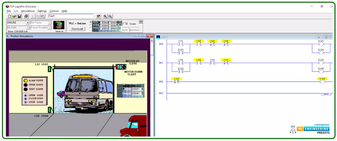
Hi Guys! hope you are doing great today! We come this time with a complete project to work out together starting from the point at which we sit with the client and receive the logical narratives that represent what they want to implement. We are going to start with a simple project this time and continue increasing the scale and complexity of the requirements through the incoming tutorials. The project we are going to implement today is one of the most common tasks that we can find in every place in our real life which is the control of the garage door. That could be found in private property or commercial buildings or public garages. Too many things need to be controlled in garage doors and several scenarios could come to your mind. However, take it as a rule of thumb that we design our program based on the requirements specified by the customer not based on our thoughts. 

Project Introduction

  Figure 1 images the project with details. As you can see, it is a garage door that is required to be controlled to open, and shut down flexibly and safely. Flexible operation means it needs to open and shut down at any time exchangeable showing operation indicators when it is opening and when it is closing. And safe operation means taking care of the motor and system components when the change between open and shut down commands for not make any kind of hazard to the system components.

Control Logic Philosophy

The control logic philosophy is a common term you will be used to hear when you meet with the clients who are going to discuss with you the control logic and all scenarios which will be interpreted by you to the control narratives. The following control narratives of the project were decided and designed based on the discussion with the customer who requested the control system and it is as follows:

  • There will be a control panel with a front panel that has push buttons, indicator lamps, and switches that enable the end user of operating the system including all functions of the control system. that includes one push button for commanding the door to open and one other push-button for instructing the system to shut down the door. In addition, one indicator to show the door is opening, one to show the door is closing, and one to show the door is in ajar status or open slightly. 

  • The system needs to have a safety emergency stop switch to stop the operation at any instant

  • The system also can switch between opening and shutting down at any time when it is allowed to do

  • The system needs to be safe and secure from any hazards that might occur due to wrong logic design for example requesting one operation which might cause any damage to the system components like motors 

  • Please note that when the customer lists the requirements he or she does not know about the deep technical details like the system components that the system needs including push buttons, indicating lamps, switches, sensors, and actuators because he or she is supposed to talk at a high level while telling you the requirements and you the one who should translate his requirements into logic narratives and deciding for the whole system components. 

Logic narratives and system components

Guys! now our work has just started by translating the above high-level requirements into detailed logic narratives and also deciding all system components and input-output lists. Figure 2 shows the garage door project with the system components that include actuators, sensors, switches, push buttons and indicator lamps.

System components

Table 1 lists the system components which include the main motor running up and down for opening and shutting down. Limit switches for preventing the door from opening and shutting down. Also, it includes the indicators and operation status while opening and closing and ajar status as well. Also, one emergency stop is utilized to stop the process at any time. The table includes the component name, description, the related IO type, and address. For example, the main motor of the door can be run in two directions to let it open or shut down. Therefore, two coils are connected through two digital outputs at addresses O:02/0 and O:02/01 which are the third output input card and the first and second channels. Also, two limit switches have been utilized to control the limits up and down to which the door can go. They are connected to two digital inputs at addresses I:01/03 and I:01/04 which are connected to the second digital input card at the 4th and 5th channels. In addition, two push buttons to handle the open and shutdown requests of the door have been connected at addresses I:01/00 and I:01/01 which are the first and second channels of the second digital input card. And the E-stop or the emergency stop has been connected to digital input at address I:01/03 which is the 4th channel of the second digital input card. Last but not least, three lamp indicators are connected via three digital outputs which are connected to addresses O:02/02, O:02/03, and O:02/04 which are the third digital output card in the rack and the third, fourth, and fifth channels respectively.

Table 1: Input-output list of the garage door project   

Component

description

IOs type

Address

Motor up 

Door motor in a clockwise direction 

Digital output

O:02/0

Motor Down

Door motor in Anticlockwise direction

Digital output

O:02/01

Limit switch

Limit switch to stop the door from over spinning

Digital input

I:01/03

Limit switch

Limit switch to stop door of over shutting down

Digital input

I:01/04

OPEN pushbutton

A pushbutton to request opening the door

Digital input

I:01/00

Shut down pushbutton

A pushbutton to request shutting the door down

Digital input

I:01/01

E-stop pushbutton

A pushbutton to request an emergency stop 

Digital input

I:01/02

Indicator lamp

Showing ajar door status

Digital output

O:02/02

Indicator lamp

Showing open door status

Digital output

O:02/03

Indicator lamp

Showing shutdown door status

Digital output

O:02/04


Project Logic Flow

Despite this is a simple and short project. And it is our first complete project. We are going systematically step by step to show you guys the right sequence to achieve a ladder logic project work. Again, we have to sit with the customer to get his requirements, and then we interpreted his requirements into a logical narrative and decided on the IOs list and all system components. Now we need to work professionally and create a flow chart that represents the program logic graphically as shown in figure 3. It shows when a request of opening the door has been requested, it checks for any emergency stop or a concurrent stop request is in progress, if no then it is clear and all set to energizing the coil of the contactors that drives the motor to run in Up direction for opening the door right away. Similarly, when a request to shut down the door. The emergency stop is checked and if is there an open door request in progress if the answer is no then it is all the settings to run the motor in the down direction to close the door by activating the related contactor to energize the motor in the direction to shut down the door.

Ladder Logic Program

Now guys after completing the design stage in which we have to design the logic and decide on the system components and the logic flow. It is time to program so let my friends open our program editor and write down the program rung by rung based on the flowchart we just have drawn in figure 3.  Looking into the ladder logic program, the first rung shows the opening handling request by energizing the output coils of the motor to run in the up direction and energizing the lamp indicator in case there is no emergency stop or a shutting down request in progress. Similarly, the second rung shows the shutdown request handling by activating the coils of the motor to run in the down direction and the indicator lamp to show the process of the shutdown of the door is in progress. That is true when there is no emergency stop is hit and no opening request is in progress. Also, you can see in both rungs for opening and shutting down the door of the garage that, the limit switches are used to prevent the door from opening or over closing for protecting the motors. At last, the third rung shows the indicator of ajar status as long as the door is not completely closed or when it is slightly opened.

Simulating the ladder logic program

Now guys! it is time to open our simulator to check if we already have written the correct logic or if there is something missed or wrong. Let me tell you something before testing your program you should hold and sit back and think about the test case scenarios for not to forget any case that might cause a failure to your program. For this very program we simulate, there are two main scenarios which are testing opening the door and testing closing the door. In addition to the main test case scenarios, there are edge test case scenarios which are testing requesting opposite operations like request opening while a shutdown process is in progress or requesting shutdown while an opening the door is in progress. Or testing requesting process while the E-stop is raised to check the safety of the operation. So let’s get started and take the test cases one by one to see if we have coded our program correctly or if there is an issue to fix.   

Testing opening the door

As you can see guys in Figure 5 in rung 2, the process of opening the door started by hitting the open push button, and because there is no emergency stop and there is no shutdown request in progress, the motor keeps spinning in the up direction and the opening lamp indicator keeps switched on. But up till when this operation will go on?

The process of opening the door is continued successfully until the LS1 is contacted at which the door has reached its final point for protecting the motor from overloading failure.

Also figure 7 shows the indicator of the door status on Ajar status whenever it is slightly opened or when it is not closed all the way.

Testing shutting down the door

Now let’s test the shutdown command by hitting the shutdown push button and notice the first rung in the program in figure 8. You can notice the door continues closing see the motor is spinning in the down direction and the indicator lamp showing closing is ON. But until when it will be stopped?

Figure 9 shows the end of the shutting down process of the door of the garage by having the limit switch LS2 reached that protects the motor from over spinning until it burned.

Testing requesting opposite operation while another is in progress

Figure 10 shows one of the edge test cases when the door was opening and all of a sudden operator requested to shut down the door. The test was successful and the operation can be reversed thanks at any time thanks to the good design by having the negative of each contact of the open and close in the other rung request as shown in rungs 1 and 2.

What’s next???

Guys! I would like to thank you all for sharing this tutorial up till this point hoping you all have enjoyed learning and practicing. And, be there with a larger project to take for the next time step by step learn, design, coding the ladder logic program, and enjoy simulating them as we are inside the factory.

Move Instruction in Ladder Logic Programming

Hi friends, today we are going to learn one of the most important instructions in the PLC ladder which is MOVE instruction by which we can move data between different memory storage including input, output, marker, and variables. Also, data of different data types and sizes can be transferred from source to destination and source memory locations. For example data types including char, string, integer, floating, time and date can be transferred between source and destination. Memory location like input, output, and marker memory area can be acting as source or destination. Furthermore, a mask can be utilized to customize and control the part of data to be transferred between source and destination. In that move with a mask, the instruction uses a source address, a destination address, and the mask as well. Guys, please do not worry if you are not understanding what is mentioned hundreds percent because you will get it in more detail and practice with the simulator as well. So let’s continue to learn and practice that MOVE and masked MOVE instruction. 

MOVE Instruction in Ladder Logic

Let’s start with the basic MOVE instruction. Figure 1 shows the typical block of a MOVE instruction in Siemens. It shows two sides for the input and output parameters of the block. Simply, the input EN input shows the contact that enables the block and triggers the movement of data between the source specified by the memory address given at input IN and the destination pointed by the memory address given at output OUT1. Also, output ENO denotes the status of the movement process to indicate the completion of the process.

Source and destination of the MOVE instruction 

As shown in the function block of the MOVE instruction shown in figure 1, there are source and destination which are an address of a memory area and can be expected to be byte, word, or double word DWORD or of any datatype like integer, character string, float, time, or date datatype. Some examples of memory size and datatype are listed in table 1 below:

Source (IN)

Destination (OUT1)

With IEC check

Without IEC check

BYTE

BYTE, WORD, DWORD

BYTE, WORD, DWORD, SINT, USINT, INT, UINT, DINT, UDINT, TIME, DATE ,TOD, CHAR

WORD

WORD, DWORD

BYTE, WORD, DWORD, SINT, USINT, INT, UINT, DINT, UDINT, TIME, DATE, TOD, CHAR

DWORD

DWORD

BYTE, WORD, DWORD, SINT, USINT, INT, UINT, DINT, UDINT, REAL, TIME, DATE, TOD, CHAR

SINT

SINT

BYTE, WORD, DWORD, SINT, USINT, INT, UINT, DINT, UDINT, TIME, DATE, TOD

USINT

USINT, UINT, UDINT

BYTE, WORD, DWORD, SINT, USINT, INT, UINT, DINT, UDINT, TIME, DATE, TOD

INT

INT

BYTE, WORD, DWORD, SINT, USINT, INT, UINT, DINT, UDINT, TIME, DATE, TOD

UINT

UINT, UDINT

BYTE, WORD, DWORD, SINT, USINT, INT, UINT, DINT, UDINT, TIME, DATE, TOD

DINT

DINT

BYTE, WORD, DWORD, SINT, USINT, INT, UINT, DINT, UDINT, TIME, DATE, TOD

UDINT

UDINT

BYTE, WORD, DWORD, SINT, USINT, INT, UINT, DINT, UDINT, TIME, DATE, TOD

REAL

REAL

DWORD, REAL

LREAL

LREAL

LREAL

TIME

TIME

BYTE, WORD, DWORD, SINT, USINT, INT, UINT, DINT, UDINT, TIME

DATE

DATE

BYTE, WORD, DWORD, SINT, USINT, INT, UINT, DINT, UDINT, DATE

TOD

TOD

BYTE, WORD, DWORD, SINT, USINT, INT, UINT, DINT, UDINT, TOD

DTL

DTL

DTL

CHAR

CHAR

BYTE, WORD, DWORD, CHAR, Character of a string1)

WCHAR

WCHAR

BYTE, WORD, DWORD, CHAR, WCHAR, character of a character string1)

MOVE instruction in ladder logic

Figure 2 shows one very basic ladder logic rung that demonstrates the usage of a MOVE instruction. It consists of a contact “trigger” to control activation of the move instruction, the MOVE instruction block which has source and destination memory address MW10 and MW12 respectively. The source and destination in this example represent integer data types.

Guys! Let's simulate this rung to learn together how the MOVE instruction works. Figure 3 shows the case when the MOVE instruction is not activated, in that case as shown in figure 3 the data is not transferred from source to destination.

But after activating the MOVE instruction by enabling the EN of the MOVE block using the contact M0.1, the data is moved from the sources to the destination.

It is important to let you guys know, this MOVE function block can be used to move different types of data types as listed above by providing the address of both source and destination.

Massive move instruction using ladder logic

Friends! Sometimes we need to move arrays of data. So do your think we are going to move one by one? The answer is yes it is possible but that is too boring to code and the program is getting very lengthy. So there is another version of MOVE instruction that enable us to move a massive amount of variables which is MOVE_BLK instruction. Figure 5 shows the function block of the massive move instruction in a very basic example ladder logic rung. As you see friends, similar to basic MOVE instruction, it has EN and ENO for enabling the instruction and returning its status showing the completion status. Also, it has an input source denoted by the address of the memory storage of the source and the address of the memory location of the destination as well. But you notice that time there is an array of variables or datatypes for source and destination. And there are other parameters called count which denotes the number of items to be moved from source to destination.  Let’s simulate this MOVE_BLK instruction to see how it works and the virtues of moving many data items in one command.

Figure 6 shows the execution having the block not activated. On the right part the memory of the source and the destination show array of 5 integers for each. You can notice guys there is no data moved.

Figure 7 shows the data is moved from source to destination after activation of the MOVE_BLK instruction. But wait for a second! Why not all the data been moved? Yes, you are correct friends, because we use count parameters to control how many variables or data items are to be transferred. And it has 3. So the first three data items have been moved only.

MOVE instruction in Allen Bradley

 Figure 8 shows a simple program that demonstrates the ladder logic rung that uses MOVE instruction. It shows the input contact I:3/0 triggers the move instruction block to activate it and enable data transfer from the 16bits input I:1 to the 16bits output O:2. On the left side, you can see guys the inputs are mirrored at the output by using the MOVE instruction. Now let’s see how we can control the data transfer using a mask to allow only selected bits to be transferred and prevent the others.

Masked move instruction

The idea behind the masked move instruction is that we utilize an array of bits to be used as a mask to filter the data that are being transferred. For example Figure 9 shows a very simple ladder logic rung that uses a masked MOVE instruction to customize the data transfer from source to destination. The MVM instruction has three parameters as shown in figure 9 which are: the source, destination, and mask. All of them are addresses of the memory area. For the very given example here, the source is the 16 bits input at I:1/0 and the output is the 16 bits output at O:2/0 while the mask is the 16bits input at I:3/0. Before we are going to simulate this example, you should expect that the data will be transferred from source to destination based on the status of every bit in the mask data.

Simulating masked move instruction

In the first test case shown in figure 10, the data to be transferred is ready at the source but nothing is transferred to the destination because the activating contact I:3/0 is not enabled. So let’s switch it on and see what is happening!

Now we enabled the activation switch at I:3/0 but still, data are not transferred from source to destination! Is there a problem in coding or logic? No, that is because the mask bits are set to off that is why bits of the source are not enabled to be transferred to the destination. Now, let us enable the masked bits and see what’s going on?

Yes! Now guys you can see all bits of the source have been transferred to the destination as long as their mates at the masked bits are enabled. But those who have their mates of bits at the mask are disabled and are still prohibited from being transferred. Like this, you can see friends how we can move data without control as when we use the MOVE instruction. In addition, you see how to control that data transfer by using mask bits as a filter. Do not forget, the move instruction can be utilized to move different data types, variables, memory sizes, and data blocks. So, it is a great tool for you as an experienced ladder logic programmer to flexibly move data between your data variables and memory location through long the program you are writing.

What’s next???

Guys! I would like to thank you for being here with me up till this point of our tutorial hoping you are really happy with it and seeing it is useful. Now guess what? I have a gift for you which is our next tutorial. It is not like every time we come up with another aspect in ladder logic to learn and enjoy practicing simulation. Now we come to the point that we should be counted as real ladder logic programmers because we have learned a lot and practiced more topics. So, it is time to practice a complete project string from reading the logic chart, understanding the logic narrative, and interpreting it to a complete successful ladder logic program. So next time will come up with a complete process with a logic diagram and requirements and practice together step by step. You can consider it as a great workshop in which you will apply all your knowledge base and what you have learned so far to take the responsibility as a PLC ladder logic programmer to convert the logic narrative and diagrams into a real ladder logic program. The work will include deciding the required logic components including switches, relays, inputs, outputs, digital and analog. Then will do a flow chart showing the logic flow based on which the program will be written. And lastly, the coded program will be applied to the plc simulator to verify the logic and make sure it is functioning correctly according to what has been requested at the beginning from the customer. So please be ready, make some revisions, and be there when we are going to learn by practicing a real project as in the real life and industry problems.

Bitwise Logic Operators in PLC Ladder Logic Programming

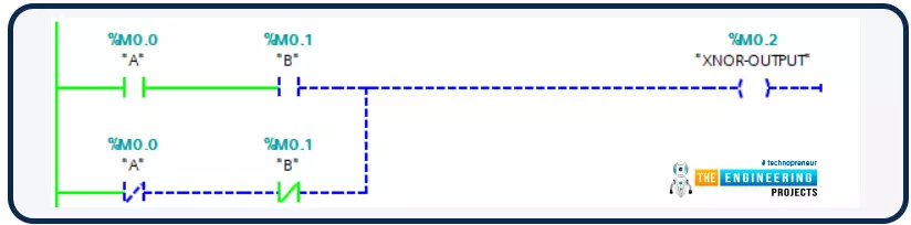
Hello friends, all of us know that PLCs are nothing but the smartest migration from relay logic control to programmable logic control. Also, you know clearly that, logic is the heart of any programming language, and the same is applied to ladder logic programming. Bitwise operators represent the logical operations including the basic logical operations like AND, OR, and NOT and the derived logical operations like NAND, NOR, and XOR. in most cases, for each bitwise operator, there are inputs based on which the output can be decided. Some of these bitwise operators have two inputs and some have only one input.  In this article, we are going to present how we can use these bitwise logical operators and their instructions with examples and practice using the PLC simulator.

Logic Gates basics and concepts

Despite we have talked about these, basics and concepts in one of our articles, we have seen it’s good to remind you briefly that basic is the ground for your foot to stand coding logical operations in ladder logic programming. for defining a logical operation, there is a truth table that shows the combinations of the inputs and the resulting output. For example, the bitwise operator that has only one input like “NOT”, has only two possible value for input which is high or low, True or False. And it has one output which is the negate of the input. So it is either TRUE or FALSE. To sum up, for every bitwise operator instruction, we are going to discuss its truth table showing the states of the possible combinations of its inputs and the resulting output as well. In addition, one example using ladder logic programming shows the operation practically. We come to see it is important to list the bitwise operators in table 1 below shows the inputs, output, and the symbol of the logical gate that is equivalent to that bitwise operator.

Table 1: the bitwise operator list 

The bitwise operator

Inputs

Output

AND

2

1

OR

2

1

NOT

1

1

NAND

2

1

NOR

2

1

XOR

2

1

AND bitwise operator

Guys, we can see the truth table of the AND instruction as tabulated in table 2. It shows the operator has two operands input A, and input B, and one output. The inputs can be switches, sensors i.e. limit switch for example while the output is a digital output to switch one actuator i.e. motor.

Input A

Input B

Output

False

False

False

True 

False

False

False

True

False

True

True

True

Also, Fig. 1 shows the symbol of the AND gate which is equivalent to AND bitwise operator. It shows two inputs A and B and only one output. Let us see that practically in ladder logic programming showing how to implement this with example.

Bitwise Operator AND in Ladder Logic

Figure 2 shows our first simple rung that codes the logic of AND bitwise logic. It shows two contacts A and B are connected in series to decide output AND-RES based on AND logic shown in truth table 2. So let us go .simulating this thing we just coded and see the logic in the application.

Simulating basic AND in ladder logic

We typically have 4 cases according to the truth table. Figure 3 shows the case when inputs A and B are low. The output shows low as shown by the coil AND-RES.

Now let us switch on input A  and keep the second operand B false as shown in fig. 4, output AND-RES output still off.

So let us try to switch the other input, B ON, and set input A off, as shown in fig. 5 output is off as represented by coil M0.2, tag AND-RES.

At last, when both inputs A and B are ON as in Fig. 6. Now only the output comes to turn ON.

Guys!, you know for sure have got to know that, with AND logic, for having the output turned high both inputs A and B must be high. 

Ladder logic in Siemens and most other brands offer the facility to perform AND between byte, word, and Double word memory space as shown in Fig. 7 shows the AND block.

Simulate AND block in ladder logic

Figure 8 shows the usage of AND block for byte data type and it is possible to do the same with a word or double word data type. The instruction block applies to byte, word, and double word data types. However, for showing one example, Fig. 8. Shows the process of byte datatype. It shows the inputs A and B represented by memory bytes MB1 and MB2 while the output is represented by MB3. The operation shown in Fig, 8, can show the AND logic between two bytes that hold values “10001110” and “00001111” so the output represented by MB3 shows the value “00001110”.

OR bitwise operator

This logic gate has two inputs and one output like the “AND” gate. Like its name, the output comes true when either input A or input B comes true as shown in Fig. 4.

Table 3 lists the truth table of the “OR” gate. It lists all possible combinations of inputs and the output status as well. It shows that the output comes to true when input A or input B comes to true.

Input A

Input B

Output

False

False

False

True 

False

True

False

True

True

True

True

True

OR bitwise in ladder logic

Figure 10 depicts the very simple rung of ladder logic that represents OR bitwise operation. It shows two inputs A and B connected in two parallel branches to give the output. So let us simulate that very OR code and apply the cases listed in the truth table in table  3.

Simulating  OR bitwise operation in ladder logic

Typically as listed in table 3, the output is low when both inputs are OFF as shown in Fig. 11.

Ohh, you can see output comes ON when input A is ON and input B is OFF as shown in Fig. 12.

Also, output comes ON when input B is ON and input A is OFF as shown in Fig. 13.

Also, you can see output comes ON when both inputs A and B are ON as shown in Fig. 14.

That concludes two things guys, in OR bitwise logic, for having output ON, there must be at least one of the inputs High. 

OR block in ladder logic

Ladder logic in Siemens and most other brands offer the facility to perform OR between byte, word, and Double word memory space as shown in Fig. 15 shows the AND block.

Simulate OR block in ladder logic

Figure 16 shows the usage of OR block for byte data type and it is possible to do the same with a word or double word data type. The instruction block applies to byte, word, and double word data types. However, for showing one example, Fig. 16. Show the process of byte datatype. It shows the inputs A and B represented by memory bytes MB1 and MB2 while the output is represented by MB3. The operation shown in Fig, 15, can show the OR logic between two bytes that hold values “00001111” and “11110000” so the output represented by MB3 shows the value “11111111”.

The bitwise “NOT”

This logic gate has only one input and one output. In a very simple language, the output is the inverted logic of the input. So when the input is true, the output would come to false and vice versa as shown in  Fig. 17.

Table 4 lists the truth table rows of all possible combinations of input and output.

Input

Output

True 

False

False

True


Figure 18 depicts a very simple example of a ladder logic rung that shows the output “NOT-A” is the negate logic of the input A.  

Simulating NOT bitwise in ladder logic

Now let's simulate the two cases listed in table 4 when inputs A is high and when it is low as well. Figure 19  and 20 show the output is the negate of the input using the NOT bitwise logic.

Now Guys we have gone through the basic bitwise logic. So how about the other bitwise logic that is formed by combining these basic bitwise operators like XNOR? let us simulate XNOR.

XNOR in ladder logic

XNOR is the negative logic of OR bitwise or you can name it as NOT-OR. Table 5 lists the combination of its two inputs and its output. It shows clearly that, the output becomes true when inputs are equal i.e. both inputs are true or both are false. Yes! Exactly, that’s why this bitwise operation is used when we need to compare two inputs if they are equal or not.

Input A

Input B

Output

0

0

1

0

1

0

1

0

0

1

1

1

Figure 21 shows the symbol of the “XNOR” logic gate showing inputs and output of the bitwise operation.

On the other hand, Fig. 22 shows a sample ladder logic of an “XNOR” logic gate implementation. It shows that there are only two ways to have the output in a TRUE state which are by set both inputs TRUE or setting both FALSE. So let us apply this to our simulator and test cases listed in table 5.

Simulating XNOR bitwise operator in ladder logic

Figure 23 shows the test of simulating XNOR when both inputs are low. You can notice friends that output comes to high.

The same thing when both inputs are high, outputs show high as shown in Fig. 24.

Ohh, you can see when one input is not matched with the other that leads to low logic of the output. That concludes the XNOR gives a high logic output when only both inputs have the same logic; otherwise, it gives a low if they are different.

What next???

Before naming the next tutorial, I would like to let you know that there are many other bitwise operators like XOR, NAND, NOR, etc. this bitwise logic can be programmed in the same scenario we demonstrated above. Now, let me tell you that the next tutorial will be about one of the most important instructions ever in the PLC that will ease the data transfer between memory locations including all data types bytes, word, Dword, etc. it is the MOVE instruction in ladder logic. So be there to learn and practice that good one.

Sequencer Output Instruction in PLC Ladder Logic Programming

Hi friends, today we are going to learn a good technique to run multi outputs in sequence. In another word, when we have some output that is repeatedly run in sequence. In the normal or conventional technique of programming we deal with them individually or one by one which takes more effort in programming and much space of memory. So instead we can use a new technique to trigger these outputs in sequence using one instruction which will save the effort of programming and space of memory. In this article, we are going to introduce how to implement sequencer output instruction. And practice some examples with the simulator as usual. Before starting the article, we need to mention that, some controllers like Allen Bradley have sequencer output instruction and some has not like Siemens. So we are going to give one example for each case showing how to code the equivalent to the sequencer output instruction in the PLCs that does not support this instruction.

Sequencer output instruction 

Figure one shows the block diagram of the process. The instruction takes the input data from the file, array, and data block and sequentially relays it to the outputs to trigger them sequentially.

Figure 2 shows the block of the sequencer output instruction showing input and output parameters. The file parameter is the first input parameter showing the address of the reference sequencer file. In addition, the mask input is to receive the address of the mask or the data block of which the instruction will move the data sequentially before relaying it to the output. Furthermore, the dest parameter is an output parameter that shows the address of the output to which the sequence bits will be applied. And the control parameter is the storage words for the status of the instruction, the file length, and the position of the pointer in the data file or array. Also, the length parameter holds the number of steps to move in the data file to the output destination sequentially. And position parameter holds the location of the pointer in the data file.


Block description and example of the sequencer output instruction

Figure 3 shows an instance of sequencer output instruction QSO. The QSO instruction steply moves through the input data file or array or data block and transfers sequentially the data bits from the data file to the output (destination word) through the mask word. The status of the instruction can be shown in the DONE (DN) bit. You should notice my friends that after the data transition is done the position is reset to the initial position or the first step.

Ladder Logic Example

Now guys, let us move to the ladder logic coding. So how does that sequencer output instruction work in ladder logic? Well!  Figure 4 shows a complete example of QSO instruction that is used in Allen Bradley to handle the sequencer output process, it shows one rung that has a start and stops push buttons from left to right at address I:0/0 and I:0/1 respectively to control the starting and stopping of the sequencer output processing. Next, you can see input I:0/2 which is used as a sequencer process flag to switch on or off the sequencer process. So, if the start PB is requested when no emergency stop and the sequencer on input is ON, the QSO is enabled and the data at address #B3:0 will be moved to dest at address O0:0 though the mask word at address 000Fh starting from position 0 with length 4.

Figure 5 shows the data file that the QSO uses to transfer sequence data bits to output. It shows the bits B3:0, B3:1, B3:2 & B3:3 are set to 1 for reference. So, when the sequencer ON input is set to high (I:0/2). The output Q:0/1 will be turned on based on the data in the data file shown in fig. 5. In that case, the length is 4 and the position is 1.

And when the sequencer flag I:0/2 is switched on next time, output O:0/2 will be switched ON. In that case, the length is 4 and the position is 2 as shown in Fig. 6.

In the third time, the sequencer flag is turned ON, the output O:0/3 will be turned ON and the length and position are updated to 4 and 3 respectively as shown in Fig. 7.

When it comes to the fourth time of switching the sequencer flag I:o/2, the output O:0/4 will be turned high and the position will be at 4 and length is 4 as shown in fig.8. At that time, the process is reset and position reset to 1.

The previous example shows how it is simple to control a bunch of outputs that are required to run in sequence with only one rung of the ladder program and using only one instruction which is QSO in Allen Bradley. This merit helps to save the memory space and time and efforts of programming and troubleshooting as well because the program will be shorter and more readable. However, still, some brands have not supported such instructions even the big names like siemens. That can not be counted as limitations but they are banking on there being a way to implement such logic. So, it is very beneficial for you guys to go implement together a piece of code (ladder logic) that is equivalent to such instruction for performing the function of sequencer output instruction in Siemens S7-1200 using our simulator. 

Ladder logic code for SQ0

As you guys see the sequencer output instruction is nothing but shifting the height value from right to left bit or right to left or even rotated shift for continuous operation. That drives our thinking to use the shift instructions in Siemens to perform this sequencer output instruction. 

Figure 9 shows the rungs of a ladder PLC simple program that implements the sequencer output process. See guys how lengthy the logic we have to code to do the same function of single instruction QSO in Allen Bradley. Again, that is a drawback or limitation thing but the program is more lengthy and takes more effort and also memory it is consuming that way. Moving to the logic listed in Fig. 9, the first thing is using a rotated shift instruction that shifts through the data block bit by bit and applies to the output QW0. At the same time increment instruction is used to move through the data. Also, one on delay timer is used to do some delay to show up the sequencing process of activating the output sequentially. And the end, a comparison instruction has been used to check if the pointer or the position reached the last output coil to reset to the first position and so on.

Simulating the sequencer output ladder code

Figure 10 shows the simulation of the sequencer output ladder code before activating the processes by using M0.0, it shows the position is at 1 and the output QW0 is all zeros. So let us activate the sequencer output process by set M0.0 to high and see the output.

Figure 11 shows the process after activating the sequencer program and starting to switch on outputs sequentially. The figure shows the process reached the sixth output coil and the position set to 7 to point at the next output. The process continues to tell reach the last one and then the position set the first step.

What’s Next???

I am glad to have you guys following tell that point and I hope you see the importance of the sequencer output technique in reducing the effort of programming and saving memory. Next time will take a tour with the bitwise logic operator and how they are utilized and how they work in the ladder program with given examples and for sure simulation to practice their usage. So let’s meet then and be ready.


Subroutine in Ladder Logic Programming

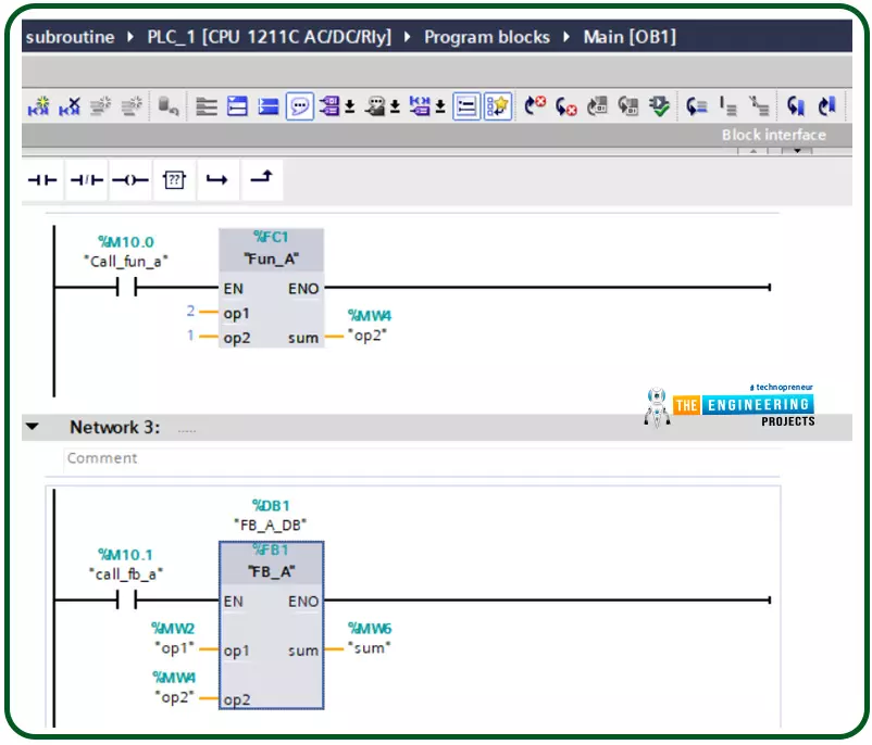
Hello friends, after completing that basic part of ladder logic programming, let us today go through one topic which is not essential to know to complete a PLC ladder program but it is important t have our code readable program and reusable pieces of code. That could happen by using what so-called a subroutine. So what is a subroutine?

Well, it is a piece of code that includes a few rungs to perform specific tasks. that piece of code can be reused numerous times through the program when we need to call it for performing that task. That subroutine enables us to structure our code like building blocks so that the program will be readable very easy and also reusable later in other projects. The idea of dividing the program into routines to apply the divide and conquer technique is very crucial to ease the coding of your program especially when it comes to the large-scale program which is the common cause in the best industry practice.

Each routine achieves one specific task and they are integrated to accomplish the whole mission. By programming in that way, the code is more readable and reusable meaning that one routine could be called many times instead of keeping repeating the lines of code or ladder rungs everywhere we need it. In this tutorial, we are going to be very familiar with subroutine-based programming including different ways to call a subroutine and the instructions that are used for handling subroutines. And yes we are going to practice examples that program that subroutines in ladder logic so let's get started.

Types of routines 

Routines can be classified into two main types: the calling routines that call subroutines. And routines that are being called. Figure 1 shows the very typical scenario of calling one subroutine. It shows the scenario when the calling routine reaches the calling instruction when the subroutine is being called with the value of the parameter passed by the calling routine and then the subroutine has a return instruction to take the execution to the following instruction of the calling instruction.  So you can imagine the calling instruction is in the calling routine which is mostly the main program and the called subroutine is responsible to return the control or the execution point to the instruction next to the calling instruction.

Passing parameters 

There are two main ways for passing parameters between the calling routine and the subroutine that is being called. The two ways are calling by value and calling by reference. In the calling by value method, the calling routine passes a copy of the original parameters so the called subroutine works on a copy. Therefore, there are no changes could happen to the original parameters in the calling routine. In contrast, in the second method which is called call by reference, the parameters are shareable between the calling routine and the subroutine that is being called. So, changes happened to the parameters but the called subroutine reflected on the original ones. Figure 2 depicts a case scenario of the two types of passing parameters. In that very example, the main routine calls subroutine “Call_Val” to apply an increment of operand “Op1” passing the parameter Op1 using the method “calling by value” while it calls “Call_ref” to do the same process but in that case, it passes parameter Op1 by using the method of “calling by reference”. As you can see, in the case it uses the “calling by value” method, it does not change the value of parameter Op1 because it uses a copy of the parameter and increments that copy not the original parameters. On the other hand, when it has used the other method, “calling by reference”, to increment the same parameter Op1, it does change the original operand because it uses a reference that points to the original parameter address. In another word, calling a subroutine based on a call by value works on a copy of the parameters and does not change the original variables while calling by reference works on the originally passed parameters so it does change the parameters. The advantage of calling by reference is saving the memory as it does not need an instance of the variables or a separate data block. On the other hand, calling by value needs to have a separate data block to include that copy of passing parameters. However, it can be called many times with a separate copy without any conflicts.

Program sequence:

Figure 3 shows the program sequence when using multilevel branching using subroutines. For example, the main module keeps carrying out the network net1, and net2, and it calls the subroutine “Sub x” in-network net3. Then subroutine “sub x ” starts executing from network net1 to net3 at which, it calls subroutine “Sub y”. Then subroutine “Sub y” carries out starting from the network “net 1”, and network “net 2” calls subroutine “Sub a”. You can notice subroutine “Sub a” returns to the calling routine “Sub y” which returns to subroutine to its calling routine “Sub x” which returns to its calling routine which is the main routine. So, you can notice how many levels of subroutine calls? Yes, they are a lot. But, it is recommended to be as much as needed for two reasons. First, many branching causes some headaches in processing in terms of memory and time. Memory is represented in the data block that is needed for each subroutine every single branching or subroutine calling and time is represented in extra instructions of calling and returning and stacking data related to the called routine and the returning addresses.

Subroutine instructions

There are two main instructions used for calling a subroutine and returning to the calling routine. Figure 4 shows the network rung that calls a subroutine called “Auto Mode”. It is going to call the subroutine at any time when the “System OK” memory contact MB180 is true. So I hope you can feel now how your program is more organized and readable when you go through the main program and easily can catch what the program does by reading the names of the called subroutines. Exactly, having a meaningful name for subroutines is very important to give the advantage of the readability of your program. So, my friends please make sure you chose a purposeful name for your subroutines.

Also fig. 5 shows the network rung that represents the returning command to the calling routine. It shows when the alarm is true represented by memory contact MB32 and pump status “Stop Pump” represented by memory bit64, the return command will be enabled for returning the execution point to the network just next to the calling network in the calling program. For example, if the calling network is at rung number 3, then the return command in the subroutine will return the execution at rung number 4 in the calling routine.  By the way, in most cases of ladder logic programming, you might not find a return instruction because it is inherently performed by completing the called subroutine but we just include it here as in fig. 5 to show up how the process of calling a subroutine and returning to the calling routine.

Figure 6 depicts the whole image of the scenario of calling one subroutine. In rung 3, a subroutine called “Auto mode” is being called by having the memory contact MB18 true. Then after that subroutine, “Auto mode” is completed it returns to the calling routine at the next rung to the calling rung which is in this case example rung number 4.  As we stated earlier, you can notice that there are now returning instructions but automatically, the called subroutine returns to the calling routine at the instruction just next to the calling instruction.

Practicing Subroutine in ladder logic

My friends, let us go to our lab as usual and do some hands-on practicing subroutine using the simulator. But before going further in practice subroutine we want to elaborate on the different types of subroutines in Siemens programming. Table 1 compares the subroutine implementation based on function and function block. It shows that subroutine can be implemented by either function FC or function block FB. And both ways can use input, output, and in-out parameters. 

FC does not use static data or data block (DB) while FB uses DB and passing parameters by making an instance of the variables which is calling by value. FC passes the parameter by pointing to the address of the variable which calling by reference technique.   

Table 1: Comparison between FC and FB subroutine in Siemens

Characteristic

FC

FB

Can be used as a subroutine

Yes

Yes

Can use parameters for Inputs, Outputs, and Input

Yes

Yes

Can use temporary variables

Yes

Yes

Can use static variables (with remanence)

No

Yes

Need an auxiliary (instance) DB for each call

No

Yes

Parameters are passed as the address for internal use

Yes

No

Parameters are copied to/from a DB (instance) for internal use

No

Yes

Can call internally a FB or FC

Yes

Yes

Can be called for a FB or FC

Yes

Yes

Can call a FB as multi-instance

No

Yes

Can be called without filling all parameters

No

Yes

Subroutine in ladder logic programming 

Again, there are two ways of calling a subroutine in Siemens ladder programming as shown in fig. 7. We have developed a sample ladder program that calls a simple subroutine to add two input operands. In the first rung, it uses function “FC1” called “fun_A” and in the second rung, it utilizes a function block FB1 called “FB_A” as you can notice function block uses a data block instance for passing a copy of the operands while function FC does not use a data block and uses the address of the input and output parameters.

Figure 8 shows the function block FB_A. the function block has two input operands which are “op1” and ‘’op2” and one output operand which is “sum”.

Because the function block passes parameters as copies or instances, fig. 9 shows the related data block DB1 which contains the parameters of the function block. It is composed of many structures for holding input, output, input, and static data as well.

On the other hand, the function uses the addresses of the parameters. Therefore, it does not need a data block as shown in fig. 10. It uses many structures to pass input, output, input, temporary, and constant data types.

Simulation work

Now let’s check the work with the simulator. Figure 11 shows the results of simulating the calling subroutine based on function FC_A that adds two static operands showing the calling path from the main organization block to the function.

On the other hand, calling a subroutine based on a function block uses an instance of parameters in a data block as shown in fig. 12. This means another instance of data is used every time we called that subroutine while using the function it is referencing the same variables at the same addresses. 

What’s next

Thank you guys for following me up to this very point of our tutorial and being very confident by knowing the subroutine you now are all set to write an organized program and readable and reusable piece of code using ladder logic programming. the next time we are going to talk about one of the most important topics in PLC programming which is master reset control showing what is it about and its importance for PLC and control project and for sure will practice with our simulator lab. So be ready and let’s meet in the next tutorial to enjoy learning and practice the PLC ladder programming series.

Master Reset Control in Ladder Logic Programming

Introduction 

Hello friends, I hope you are doing very well. Today we are going to learn and practice the master control reset (MCR)! So what is that MCR? Well! This is a tool you might use to control a group of devices with one push button for performing fast emergency responses with one click for a group of devices in one zone. In another word, you divide the program into zones and put this zone between a master control to control their operation as one unit by one contact. This technique is useful for applying emergence stops and also protecting some equipment by applying a safety restriction to not operate when that condition is in effect. 

The concept of the master control reset (MCR)

Figure 1 shows the master control relay in a ladder logic showing a couple of rungs between the master control and master control reset to be controlled as one zone by master control. for example, input 1 enables the master control relay M100 which is the only way to relay the hotline of power to rungs 2 and 3 as shown in the figure. When input 1 is on, the master control relay is energized. Therefore, input 2 and input 3 can energize output 1 and output 2 respectively. But, if input 1 is off, the master control relay is off. Therefore, rungs 2 and 3 are disconnected from the power. Therefore, even if input 2 and input 3 are on, outputs 1 and 2 will not energize because of a missing connection to power via master control relay M100. To sum up, there is a zone that contains a couple of rungs, these rungs are not enabled without master control enabled. Also, fig. 1 shows the structure of the master control and master control reset to have one rung to enable the master control relay and one rung at the end to represent the master control reset and declare the end of the zone that is under master control. and the code or rungs that are located between the master control and the master control reset is the zone that we need to control its running based on master control. So, if the master control is not true, the code in that zone between the master control and the master control reset will be bypassed and the next instruction after the master control reset instruction will be executed. 

The concept looks very simple but it is crucial for safety and control techniques. Also, many master control and zones can have in our program as shown in fig. 2. It shows more than one zone and each one is controlled by its master control.

So we want to go further in demonstrating the master control reset by a practical example from real life. Figure 3 shows a practical example of real-life in the industry of which automatic bottle filling process. So what does master control have to do with such a process? Will! That is a good question because it tells me you understand master control reset and are with me on the same page. So, as you can see, there is the start and stop pushbuttons and we need to use master control to control starting and stopping the whole process regardless of the status of individual inputs and sensors. by having such control, we can stop the process in any emergency case or for doing maintenance. The sequence of the process is to start moving the conveyor by hitting the start push button. The conveyor keeps running until the proximity sensor comes ON. At that time, the valve will open for 5 seconds and then the conveyor continue moving again after 5 seconds and continue for 3 bottles repeating the same process. But if there is an emergency happens, there should be a way to stop the process including moving the conveyor, and opening the valve even if all conditions to do are met. Well done! You are correct, master control and master control reset should bracket the process to be enabled and disabled when that emergency comes to happen.

Master control in ladder logic

Master control and master control reset are the same concepts. However, a few differences you can notice in ladder logic from one plc brand to another. For example, Fig. 4 shows the ladder logic code of a master control reset in Mitsubishi PLC. You can notice the same concept has been applied. A zone of a couple of rungs is surrounded by master control and master control reset instructions based on master control relay M100. Input 1, X400 enables the master control relay M100. And rungs 2 and 3 are included in the zone under master control.

On the other hand, master control and master control reset look a little bit different in Allen-Bradley as shown in fig.5. However, you can notice the same concept is applied by having the zone that includes a couple of rungs between the master control relay and master control reset for enabling or disabling that zone based on the logic and situation.

Also, Siemens shows a few differences in ladder logic of master control as shown in Fig.6. however, the same concept is thereby enclosing the code to be controlled in a zone preceded by enabling to master control relay and followed by a master control reset to clear that master control and show the end of the controlled zone.

Practice Ladder logic example

Guys, it is now the time to enter our lab and enjoy practicing the master control and master control reset by using our simulator as usual for validating our understanding of what we have gone through in this tutorial on ladder logic programming. In the example simulated below and shown in fig. 7, we have designed simple master control and master control rest to have master control of running of Q0.0. you can notice that, despite input I0.1 being true, Q0.0 is not energized because master control is not enabled or in off status. So what happens if we enable master control by switching on input I0.0?

Yes, you are correct! The output Q0.0 will now work after enabling the master control by turning input I0.0 on as shown in Fig.8.

What’s next???

Let me thank you guys for following up until this point and because your knowledge of ladder logging is getting increase every single tutorial, I would like to announce that, the next tutorial will be about one of the very advanced levels of ladder logic programming which is for expert and I thought you are now. The sequencer output instruction in ladder logic is our topic for the next tutorial in which we will learn and practice how to, massively output data sequentially to outputs. Please do not worry if that is not clear for now and just be there to go through it step by step and enjoy practicing one topic for an expert ladder programmer.

Syed Zain Nasir

I am Syed Zain Nasir, the founder of <a href=https://www.TheEngineeringProjects.com/>The Engineering Projects</a> (TEP). I am a programmer since 2009 before that I just search things, make small projects and now I am sharing my knowledge through this platform.I also work as a freelancer and did many projects related to programming and electrical circuitry. <a href=https://plus.google.com/+SyedZainNasir/>My Google Profile+</a>

Share
Published by
Syed Zain Nasir