Interface 7-Segment Display with Raspberry Pi 4

Thank you for being here for today's tutorial of our in-depth Raspberry Pi programming tutorial. The previous tutorial taught us how to install a PIR sensor on a Raspberry Pi 4 to create a motion detector. However, this tutorial will teach you how to connect a single seven-segment display to a Raspberry Pi 4. In the following sections, we will show you how to connect a Raspberry Pi to a 4-digit Seven-Segment Display Module so that the time can be shown on it.

Seven-segment displays are a simple type of Display that use eight light-emitting diodes to show off decimal numbers. It's common to find it in gadgets like digital clocks, calculators, and electronic meters that show numbers. Raspberry Pi, built around an ARM chip, is widely acknowledged as an excellent Development Platform. Its strong processing power can do amazing things in the hands of electronics enthusiasts and students. If we can figure out how to have it talk to the outside world and process data via an output, then we'll have a real chance of accomplishing all this. We analyze the data by viewing it on an LCD screen or other Display. Numerous sensors can detect specific parameters in the physical world and convert them to the digital world. It would never make sense to utilize a PI LCD panel to display a minimal quantity of information. Here, a 7-Segment or 16x2-Alphanumeric LCD panel is the preferred method of presentation.

There are few uses for a 7-segment display that don't need an LCD panel, even though a 16x2 LCD is preferable in most. If all you need to do is show some numbers, then an LCD, which has the downside of having a small character size, is excessive. Compared to a regular LCD screen, seven segments have the upper hand in dim environments and can be seen from wider angles. Let's get started.

Where To Buy?
No.ComponentsDistributorLink To Buy
1BreadboardAmazonBuy Now
2Jumper WiresAmazonBuy Now
3Raspberry Pi 4AmazonBuy Now

Components

  • Jumper wires

  • Seven segment display

  • 1KΩresistors

  • Breadboard

The 7-Segment and 4-Digit Display Modules

The seven segments of a 7 Segment Display are each lit up by an individual LED to show the digits. To show the number 5, for example, you would make the glow pins for segments a, f, g, c, and d on the 7-segment high. This particular 7-segment display is a Common Cathode version, although there is also a Common Anode version.

One 7-Segment Display Interfacing with Pi 4

The wiring diagram for connecting a 7-segment display to a Raspberry Pi is shown below. Here, 7-Segment Common Cathode has been utilized.

So, we'll simulate an 8-bit PORT on PI using its eight GPIO pins. Here, GPIO12 is the Most Significant Bit (MSB), while GPIO13 is the Least Significant Bit (LSB) (Most Significant Bit).

If we wish to show the number 1, we must activate both segments B and C. We must supply voltage to GPIO6 and GPIO16 to power segments B and C. Accordingly, the hexadecimal value of "PORT" is "06," and the byte value of "PORT" is "0b00000110." If we raise both pins to their highest positions, the number "1" will be shown.

The value for every displayable digit has been recorded and saved in a Character String with the label 'DISPLAY .'We have then used the Function 'PORT' to call those values one at a time and display the relevant digit.

Explanation of the Code

Once everything is wired up according to the schematic, we can power up the PI and begin using PYTHON to write the program. Below is a function that allows us to program the GPIO pins on the PI, and we'll go over the few commands we'll be using in the PYTHON program to do so. We are also changing the name of the GPIO pins in the hardware from "GPIO" to "IO," which will be used throughout the code.

import RPi.GPIO as IO

The general-purpose input/output (GPIO) pins we need to use may be occupied with other tasks. If that's the case, the program's execution will be interrupted by warnings. The below command instructs the PI to continue running the software regardless of the warnings.

IO.setwarnings(False)

Pin numbers on the board and pin functions can be used to refer to PI's GPIOs. This GPIO5 is similar to the one labeled "PIN 29" on the board. Here we specify whether the number 29 or the number 5 will stand in for the pin.

IO.setmode (IO.BCM)

To use the LCD's data and control pins, we have assigned those functions to eight of the GPIO pins.

IO.setup(13,IO.OUT)

IO.setup(6,IO.OUT)

IO.setup(16,IO.OUT)

IO.setup(20,IO.OUT)

IO.setup(21,IO.OUT)

IO.setup(19,IO.OUT)

IO.setup(26,IO.OUT)

IO.setup(12,IO.OUT)

If the condition between the brackets evaluates to true, the looped statements will be run once. The value of PIN13 would be HIGH if and only if bit0 of the 8-bit 'pin' is true. There are eight 'if else' conditions, one for each of bits 0 through 7, so that each LED in the seven-segment Display can be set to either the High or Low state, depending on the value of the corresponding bit.

if(pin&0x01 == 0x01):

   IO.output(13,1)

else:

   IO.output(13,0)

As x increases from 0 to 9, the loop will be run 10 times for each command.

for x in range(10):

The following command can create an infinite loop, with which the statements included within the loop will be run repeatedly.

While 1:

All other commands and functions have been commented on in the following code.

Single 7-segment Display complete code

import RPi.GPIO as IO            # calling for the header file, which helps us use GPIO's of PI

import time                              # calling for time to provide delays in the program

DISPLAY = [0x3F,0x06,0x5B,0x4F,0x66,0x6D,0x7D,0x07,0x7F,0x67]            # string of characters storing PORT values for each digit.

IO.setwarnings(False)            # do not show any warnings.

IO.setmode (IO.BCM)           # programming the GPIO by BCM pin numbers. (like PIN29 as‘GPIO5’)

IO.setup(13,IO.OUT)             # initialize GPIO Pins as outputs

IO.setup(6,IO.OUT)

IO.setup(16,IO.OUT)

IO.setup(20,IO.OUT)

IO.setup(21,IO.OUT)

IO.setup(19,IO.OUT)

IO.setup(26,IO.OUT)

IO.setup(12,IO.OUT)

def PORT(pin):                    # assigning GPIO logic by taking the 'pin' value

    if(pin&0x01 == 0x01):

        IO.output(13,1)            # if  bit0 of 8bit 'pin' is true, pull PIN13 high

    else:

        IO.output(13,0)            # if  bit0 of 8bit 'pin' is false, pull PIN13 low

    if(pin&0x02 == 0x02):

        IO.output(6,1)             # if  bit1 of 8bit 'pin' is true, pull PIN6 high

    else:

        IO.output(6,0)            #if  bit1 of 8bit 'pin' is false, pull PIN6 low

    if(pin&0x04 == 0x04):

        IO.output(16,1)

    else:

        IO.output(16,0)

    if(pin&0x08 == 0x08):

        IO.output(20,1)

    else:

        IO.output(20,0)   

    if(pin&0x10 == 0x10):

        IO.output(21,1)

    else:

        IO.output(21,0)

    if(pin&0x20 == 0x20):

        IO.output(19,1)

    else:

        IO.output(19,0)

    if(pin&0x40 == 0x40):

        IO.output(26,1)

    else:

        IO.output(26,0)

    if(pin&0x80 == 0x80):

        IO.output(12,1)            # if  bit7 of 8bit 'pin' is true, pull PIN12 high

    else:

        IO.output(12,0)            # if  bit7 of 8bit 'pin' is false, pull PIN12 low

While 1:

    for x in range(10):            # execute the loop ten times incrementing x value from zero to nine

        pin = DISPLAY[x]        # assigning value to 'pin' for each digit

        PORT(pin);                  # showing each digit on display 

        time.sleep(1)

Output

The process of displaying a single number character on a 7-segment display is complete. However, we'd need more than a single 7-segment display to express information with more than one digit. Therefore, we will use a 4-digit seven-segment display circuit for this session.

Four individual Seven-Segment Displays have been linked up here. For a 4-digit 7-segment display, we know that each module will have 10 pins, so there will be 40 pins total. Soldering that many pins onto a dot board would be a hassle for anyone; thus, I recommend that anyone using a 7-segment display do so by purchasing a module or creating their PCB. See below for a diagram of the relevant connections:

In the preceding diagrams, we can see that the A-lines of all four displays are linked together as one A, and the same is true for B, C.... up until DP, which is essential for understanding how the 4-digit seven-segment module functions. Put another way, if trigger A is activated, the state of all 4 A's should be high.

Nonetheless, this never occurs. The four extra pins labeled D0 through D3 (D0, D1, D2, and D3) let us select which of the four displays is driven high. As an illustration, if I want my output to appear solely on the second Display, I would set D1 to high and leave D0, D2, and D3 at low. Using pins D0–D3 and A–DP, we can easily choose which displays should be on and which characters should be shown.

Using a Pi 4  to interface with a 4-digit, 7-segment display module

Let's check the many options for interfacing this 4-digit seven-segment Display with the Raspberry Pi. As can be seen in the diagram below, there are 16 pins on the 7-segment module. Even if your module's resources are limited, it will provide at least the following.

  • Segmented pins, either 7 or 8 segments (pins 1 to 8)

  • Pin holder to the ground (here pin 11)

  • A 4-digit code to unlock the door (pins 13 to 16)

See below for the wiring diagram of a digital clock built with a Raspberry Pi and a 4-digit Seven-segment display module:

You can also use the following table to ensure your connections are correct and follow the diagrams.

Locating the module's pins is the first step in making electrical connections. Identifying the Raspberry Pi's GPIO pins can be tricky; I've included an image to help.

Raspberry Pi programming

Here, RPi is programmed in the Python programming language. The Raspberry Pi can be programmed in a wide variety of ways. Since Python 3 has become the de facto standard, we've opted to use that version as our integrated development environment (IDE). At the bottom of this guide, you'll find the whole Python code.

We'll go over the PYTHON instructions we'll be using for this project: first, we'll import the library's GPIO file; next, using the below function, we'll be able to program the Pi 4's GPIO pins. We are also changing the name of the GPIO pins in the hardware from "GPIO" to "IO," which will be used throughout the code. We've brought in time and DateTime to get the current time from Rasp Pi.

import RPi.GPIO as GPIO

import time, DateTime

The GPIO pins we're trying to use are already being used for something else. The program's execution will be interrupted with warnings if this is the case. The PI will be instructed to disregard the errors and continue with the software using the below command.

IO.setwarnings(False)

The physical pin number and the corresponding function number can refer to PI's GPIOs. As with 'PIN 29,' GPIO5 is a physical component on the circuit board. In this case, we specify whether the number "29" or "5" will stand in for the pin. GPIO. In BCM notation, GPIO5 pin 29 will be represented by a 5.

IO.setmode (GPIO.BCM)

As is customary, we'll start by setting the pins to their default values; in this case, both the segment and digit pins will be used as outputs. In our code, we organize the segment pins into arrays and set their values to zero by declaring them to be GPIO.OUT.

segment8 = (26,19,13,6,5,11,9,10)

for segment in segment8:

    GPIO.setup(segment, GPIO.OUT)

    GPIO.output(segment, 0)

We do the same thing with the digital pins, but we set them to output and set them to zero by default.

#Digit 1

    GPIO.setup(7, GPIO.OUT)

    GPIO.output(7, 0) #Off initially

    #Digit 2

    GPIO.setup(8, GPIO.OUT)

    GPIO.output(8, 0) #Off initially

    #Digit 3

    GPIO.setup(25, GPIO.OUT)

    GPIO.output(25, 0) #Off initially

    #Digit 4

    GPIO.setup(24, GPIO.OUT)

    GPIO.output(24, 0) #Off initially

Numbers on a seven-segment display must be formed into arrays. To show a single digit, we need to toggle the on/off status of all but the dot pin of the 7-segment Display. For the numeral 5, for instance, we can use this setup:

For all alphabets and numerals, there is an equivalent sequence number. You can write on your own or utilize the handy table provided.

Using this information, we can create arrays for each digit in our Python code, as demonstrated below.

null = [0,0,0,0,0,0,0]

zero = [1,1,1,1,1,1,0]

one = [0,1,1,0,0,0,0]

two = [1,1,0,1,1,0,1]

three = [1,1,1,1,0,0,1]

four = [0,1,1,0,0,1,1]

five = [1,0,1,1,0,1,1]

six = [1,0,1,1,1,1,1]

seven = [1,1,1,0,0,0,0]

eight = [1,1,1,1,1,1,1]

nine = [1,1,1,1,0,1,1]

Let's bypass the function in the code that would otherwise be executed before entering the while loop and begin displaying characters on our 7-segment Display. If you hook up a Raspberry Pi to the internet, it will read the current time and divide it into four separate variables. For instance, when the time is 10.45, the values assigned to h1 and h2 will be 1 and 0, while m1 and m2 will be 4 and 5, respectively.

now = DateTime.DateTime.now()

    hour = now.hour

    minute = now.minute

    h1 = hour/10

    h2 = hour % 10

    m1 = minute /10

    m2 = minute % 10

    print (h1,h2,m1,m2)

These four numbers will be displayed on one of our four digits. The lines below can be used to convert a variable's value to a decimal. Here, we show the value in variables on the 7-segment Display by using the function print segment (variable) with the digit 1 set to the highest possible value. You may be asking why we turn off this digit and why there's a delay after that.

GPIO.output(7, 1) #Turn on Digit One

print_segment (h1) #Print h1 on segment

time.sleep(delay_time)

GPIO.output(7, 0) #Turn off Digit One

This is because the user will only be able to see the full four-digit number if all four digits are shown at once, and we all know that this isn't possible.

How, then, can we simultaneously show all four digits? With luck, our MPU is considerably quicker than the human eye. Therefore we offer one number at a time but exceptionally quickly. The MPU and segment display are given 2ms (variable delay time) to process each digit before we go on to the next. A human being cannot detect this 2ms lag; therefore, it appears as though all four digits illuminate simultaneously.

Understanding how to use print segment(variable) is the final puzzle piece. Arrays that have been declared outside of this function are used within it. As a result, the value of any variable passed to this function must be inside the range (0-9) so that the character variable can use in a meaningful comparison. Here, we check the variable against the value 1. The same is true for all comparisons with numbers between zero and nine. Assigning each value from the arrays to the appropriate segment pins is what we do if a match is found.

def print_segment(character):

    if character == 1:

        for i in range(7):

            GPIO.output(segment8[i], one[i])

Show the time on a 4-digit 7-segment display.

Use the provided schematic and code to connect your components and set up your Raspberry Pi. Once you've finished setting everything up, you can open the software and check the 7-segment Display to see the time. However, before doing this, you should check a few things.

  • If you want to be sure your Raspberry Pi isn't stuck in the past, you should update its time.

  • If you want to utilize a 7-segment display on your Raspberry Pi, you'll need to plug it into an adapter rather than a computer's USB connection because of the large amount of current it consumes.

Complete code

import RPi.GPIO as GPIO

import time, DateTime

now = datetime.datetime.now()

GPIO.setmode(GPIO.BCM)

GPIO.setwarnings(False)

 #GPIO ports for the 7seg pins

segment8 =  (26,19,13,6,5,11,9,10)

for segment in segment8:

    GPIO.setup(segment, GPIO.OUT)

    GPIO.output(segment, 0)

    #Digit 1

    GPIO.setup(7, GPIO.OUT)

    GPIO.output(7, 0) #Off initially

    #Digit 2

    GPIO.setup(8, GPIO.OUT)

    GPIO.output(8, 0) #Off initially

    #Digit 3

    GPIO.setup(25, GPIO.OUT)

    GPIO.output(25, 0) #Off initially

    #Digit 4

    GPIO.setup(24, GPIO.OUT)

    GPIO.output(24, 0) #Off initially

null = [0,0,0,0,0,0,0]

zero = [1,1,1,1,1,1,0]

one = [0,1,1,0,0,0,0]

two = [1,1,0,1,1,0,1]

three = [1,1,1,1,0,0,1]

four = [0,1,1,0,0,1,1]

five = [1,0,1,1,0,1,1]

six = [1,0,1,1,1,1,1]

seven = [1,1,1,0,0,0,0]

eight = [1,1,1,1,1,1,1]

nine = [1,1,1,1,0,1,1]

def print_segment(charector):

    if charector == 1:

        for i in range(7):

            GPIO.output(segment8[i], one[i])

    if charector == 2:

        for i in range(7):

            GPIO.output(segment8[i], two[i])

    if charector == 3:

        for i in range(7):

            GPIO.output(segment8[i], three[i])

    if charector == 4:

        for i in range(7):

            GPIO.output(segment8[i], four[i])

    if charector == 5:

        for i in range(7):

            GPIO.output(segment8[i], five[i])

    if charector == 6:

        for i in range(7):

            GPIO.output(segment8[i], six[i])

    if charector == 7:

        for i in range(7):

            GPIO.output(segment8[i], seven[i])

    if charector == 8:

        for i in range(7):

            GPIO.output(segment8[i], eight[i])

    if charector == 9:

        for i in range(7):

            GPIO.output(segment8[i], nine[i])

    if charector == 0:

        for i in range(7):

            GPIO.output(segment8[i], zero[i])               

    return;

while 1:

    now = DateTime.DateTime.now()

    hour = now.hour

    minute = now.minute

    h1 = hour/10

    h2 = hour % 10

    m1 = minute /10

    m2 = minute % 10

    print (h1,h2,m1,m2)

    delay_time = 0.001 #delay to create the virtual effect

    GPIO.output(7, 1) #Turn on Digit One

    print_segment (h1) #Print h1 on segment

    time.sleep(delay_time)

    GPIO.output(7, 0) #Turn off Digit One

    GPIO.output(8, 1) #Turn on Digit One

    print_segment (h2) #Print h1 on segment

    GPIO.output(10, 1) #Display point On

    time.sleep(delay_time)

    GPIO.output(10, 0) #Display point Off

    GPIO.output(8, 0) #Turn off Digit One

    GPIO.output(25, 1) #Turn on Digit One

    print_segment (m1) #Print h1 on segment

    time.sleep(delay_time)

    GPIO.output(25, 0) #Turn off Digit One

    GPIO.output(24, 1) #Turn on Digit One

    print_segment (m2) #Print h1 on segment

    time.sleep(delay_time)

    GPIO.output(24, 0) #Turn off Digit One

    #time.sleep(1)

Output

A similar section should appear below if everything is functioning as it should.

7-segment Display limitations

Typically, only 16 hexadecimal digits can be shown on a seven-segment display. Some show the digits 0-9, whereas others can show more. Seven-segment displays can only show a maximum of 16 values due to a lack of input leads. However, LED technology does allow for more than this. Even with the help of integrated circuit technology, the possible permutations of the seven parts on the screen are very few.

Conclusion

This guide taught us how to connect a 7-segment screen to a Raspberry Pi 4. The seven-segment Display, which we learned is employed in digital timers, clocks, and other electrical gadgets, are a cheap, basic electrical circuit and reliable module. Seven-segment displays can either be "common-anode" (where the common point is the power input) or "common-cathode" (where the common end is grounded). After that, we coded some python scripts to show numbers on a single seven-segment model and the time across four such screens. Next, we'll see how to use a Raspberry Pi 4 as the basis for a low-power Bitcoin miner.

Getting Past Legacy Software Pains in Requirements Management

Legacy software refers to a business operating software that has been in use for a long time. This is older system software that is still relevant and fulfills the business needs. The software is critical to the business mission and the software operates on specific hardware for this reason.

Generally, the hardware in this situation has a shorter lifespan than the software. With time, the hardware becomes harder to maintain. Such a system will either be too complex or expensive to replace. For that reason, it continues operating.

What is a Legacy System?

Legacy software and legacy hardware are often installed and maintained simultaneously within an organization. The main changes to the legacy system typically only replace the hardware. That helps to avoid the onerous requirements management of the software certification process.

Which Businesses Have Legacy Systems?

Legacy systems operate in a wide range of business organizations, such as banks, manufacturing, energy companies, hospitals, and insurance companies. You can also find them in the defense industry, among other multifaceted business organizations.

Legacy Software Pains in Requirements Management

Only companies born in the digital age don't face the problem of chronic legacy system pains, i.e. the distress of a lack of digital transformation. Legacy systems can involve unbearable complexity, mismatched skills, lack of innovation, bureaucracy, and so on.

Legacy systems form in organizations for many reasons. First, compliance issues and a rollout are often challenging to carry out all at once. There may be an ongoing project that needs the old system. There are also instances where decision-makers don't like change.

However, the shortcomings of operating an old system are annoying and can also cause severe damage to the company. The pains of operating an old system include:

Legacy Systems Strategies are Not Prepared For Change

Legacy systems can include the 'Stop and Start' strategy. There are also long static periods or unchanging business, which was the mainstream way of running business operations throughout the industrial age. This means systems have a short period to make and adapt to any necessary changes, while business stops and waits for the wave of essential changes to finish.

The world doesn't work like this anymore. Intermittent changes allow organizations with old systems to persist up to the next phase of evolution.

Fortunately, there is an alternate option called lean IT. The model advocates for making positive changes and continuous improvements and is aimed at avoiding getting stuck in waiting mode.

The lean IT model is well suited to data-oriented and digital systems, and helps discourage the myopic views that legacy systems foster in the first place.

Legacy Systems Create Security Problems

Legacy systems can pose several data security problems in an organization. Security is a prominent feature of the lean IT model. Continuous improvements and positive changes help to curb the latest threats. Old systems, because of their age, struggle with this.

Legacy systems may pose various challenges when fixing specific vulnerabilities, due to their large and inflexible nature. Making a fix in legacy systems can face delays because developers find it challenging to create one. Also, creating a repair is often not on the development team’s priority list. As a result, the fix ends up being very expensive.

Old systems can enter into a period where there is a danger to the organization due to their outdated security measures.

Inability to Meet Customers on Their Terms

The digital age has created tremendous opportunities, including those related to changing a company's way of operations to benefit its users. Businesses that don't have legacy systems find that when technology moves, the industry can move with it. They are ready to use any new generation that comes out and are prepared to download and install any new application that becomes popular.

Under these conditions, challenges can mount for a company stuck with an old system. Legacy systems have restrictions on using new applications. Businesses that have many customer interactions can encounter serious challenges.

Customers often go for features on the latest applications available in this digital era, such as Instagram and Windows 10 updates. Both of these have chatting options that legacy systems can't enable. This is very much a missed opportunity.

Legacy Systems are Not Cost Effective

It may seem like legacy systems would be less expensive to maintain. However, that connotation changes over time, and circumstances often prove cost to be a pain point. Support and software updates for legacy systems are often much more expensive than current models, whose support and updates are always ready for seamless implementation.

The reason behind the additional maintenance cost is that knowledgeable software developers are hard to find. It involves a lot more work for software developers to offer the necessary continued care and updates for a legacy system than a current system.

Compatibility Issues Threaten Business Interaction

A legacy systems compatibility issue affects all users. We’re talking about the customers and business partners, suppliers, team members, and other associated users.

The legacy system will support file and data formats up to a certain point. But over time, these formats advance over and beyond what the legacy system can handle.

The evolution of support formats only takes a couple of years. In this event, the business will be stuck and experience pain points from using forms the customers or partners are no longer willing to use.

A company without legacy problems will adapt to successful implementation fast, aiming for better collaborations among users and team members. They also avoid waste in IT operations. Therefore, the future of the company's business remains adaptable.

Lack of Storage Availability and Budget

Legacy systems are often full of lurking, untested problems. Support is often difficult to come by, leading to frustrating support interactions.

Customer support is critical, especially when you have large data sets or tight deadlines. Modern software development techniques make it easy to release and access track records. System data storage matters a lot to the users, so data storage and accessibility are key features in new systems that also come in handy when support is necessary.

Unhealthy for Employee Training

Look at the IT team members' psychological aspects for a moment. What does operating a legacy system say to the workforce? It signals that it's okay to work with an old system on one end while putting off addressing worries until later. The system solutions from the past are still working.

But an organization should not encourage this view in their employees, especially when training employees in new skills.

The method may still function, but it will be a massive liability for connectivity and security. Legacy systems also reduce productivity, lower team members' morale, and repel some of the best talents. Employees with first-hand experience in new technology want to hold to that and have no interest in learning old systems.

"If it's not broken, don't fix it" is the IT professional's general attitude. Though it does not stem from any bad intentions, it can cause a company severe problems down the road.

Proprietary Tools are Not Fun

Legacy systems tend to be clunky, extensive, and very proprietary. Changing or customizing them poses a serious challenge. But modern IT professionals prefer to use the latest techniques and have no interest in mastering old systems.

Some organizations' software and hardware needs are different from other companies. Therefore, they need to build their custom software and hardware. New systems have smaller parts that make them flexible and easy to adopt. Specialized needs are no excuse for retaining legacy systems.

Getting Past Legacy Software Pains In Requirements Management

High-regulated industries have difficulty catching up with technology because of their complex systems. You may feel your company has outgrown its requirements management software, and you’re not alone.

The line between software and hardware becomes more and more blurred, and innovations are occurring faster than ever before. Requirements management providers may not supply the right software that matches the users' goals, regardless of the notable reputation or how complex the software is. That can create severe problems that affect productivity.

Here are some common methods for how to work your way out from a legacy system into something much more helpful for yourself and your customers:

Working with Multiple Stakeholders in Mind

Highly regulated industries interact with many different stakeholders and players, which is good for their business. It is essential to value the input of the various roles and skill sets.

But problems can arise if one of these users doesn't know how to use your requirements management software. Stakeholders bring their benefits to the company, but interfering with the system can be a recipe for compliance disaster.

To avoid such problems, look for software that flows with several roles and is seamless. Also, make sure your software integrates user-friendly traceability. Every user on the project needs to see the progress from beginning to end. This will prevent use problems from becoming a lasting problem and hindering productivity.

Timely Notifications to Help Meet Deadlines

Missing deadlines happen in many organizations. A team member needs to provide feedback but fails to do so on time. It could have been sent via email, Google, or Word document that someone didn’t know to monitor. Whichever means were used, the model of collaboration in place failed.

Review processes are quite complex these days, and you need collaboration software that sets clear intentions for the users. Real-time notification and editing will help keep team members on the truck.

Opt for a requirements management tool that prompts the next step to avoid falling into the trap. The requirements management software will help to prevent blame games - and it’s an excellent reason to suggest upgrading away from the legacy system altogether.

Accessibility and Intuitiveness

There may be instances where you want to carry out an essential process through the legacy system - but you are somehow locked out. You may have challenges finding the person who manages the system access rights and can get you back in the loop.

The situation can be frustrating and pose significant risks to the company, since one can attempt to break into the system for a couple of hours. This also wastes time. The desire to provide timely feedback with confidence is thwarted, which goes against the first intention of collecting the data.

The right requirements management tool should provide continuous data collection and growth. To achieve this, it should be open, accessible, and intuitive. The stakeholders will get motivation and provide constant input and collaboration, which is vital in keeping up with breakneck innovation.

An Upgrade Doesn’t Have to Spell Disaster

When an upgrade notification pops up on our screen, it’s normal to get skittish. There was once a very real fear of losing essential data and vital information with any kind of system update.

But this fear has dissipated with the advent of the cloud. A company no longer has to fear upgrading and fixing software requirements. It’s necessary to improve the security requirements and access some of the latest features.

It's crucial to have a system that adapts quickly to update requirements. When purchasing legacy software, consider the opportunity costs of not upgrading and encountering the headache of being locked out of various unsupported platforms.

Data Storage, Security, and Availability

As part of evaluating your current system, investigate data storage safety during software development. Find out from existing customers how well your system releases the accurate document.

Whatever system you choose will be around for a long time, so you will need to measure your predicted needs from the vendor. You will be putting some of your crown jewels on the system you want to buy. They need to be safe.

Conclusion

We live in an age with the most innovative and disruptive products available to more people than ever. We have ultra-fast electric cars, self-piloted spaceships, and lifelike prosthetics. We also have some of the brightest minds toiling to help propel us into the future.

This means the regulatory environment now is more stringent, especially on public safety and the marketplace demands. There is a need to have a team ready to meet the ever-increasing demands of compliance.

To be on the safer side, you need to put in place a collaborative infrastructure to keep the team organized and detect mistakes of disconnected persons in real-time. The future of your company depends on it.

Frequently Asked Questions

In what ways can one modernize a legacy system?

Migrate. This allows the business to perform critical processes immediately. Legacy software may not be flexible enough to allow the expected modification. Also, your old system may not offer its users the right results. Legacy migration can be the better choice in this case.

The other option is extension. You may not need to replace a legacy system that still performs its core functions (especially if it still has some years of warranty remaining). Despite that, you can still modernize it by extending its capabilities.

How do you handle management pushing legacy systems?

Try to make concrete and practical recommendations on how to make the legacy system better. Provide evidence on how the improvements will lead to better performance. You may change minds by presenting realistic situations where the legacy system can still be helpful in the future with just a few additions.

Up Down Counter without Microcontroller

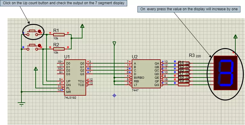
Hello geeks, welcome to our new project. In this project, we are going to make a very interesting project. I think most of us have seen the scoreboards in sports, after looking at that, have you ever wondered about the working of it. Therefore, this time, we will be making something like that only with some extra features. So basically that score board is nothing but a counter which counts the scores. Most of the geeks who have an electronics background or have ever studied digital electronics must have heard about the counter.

Here, in this project, we are going to make an Up-Down counter. A simple counter counts in increasing or decreasing order but the Up-Down counter counts in increasing and decreasing order, both depending upon the input it has given.

But I am having an interesting question about the counter. Let suppose if the counter is counting in increasing order then up to which value, it will count because it can not count to infinite which means it has to reset after some certain value, and I believe that you must be having the same doubt as well. Basically every counter resets itself after a certain value and that value depends upon the bits of a counter.

Let suppose, we have a 8 bit counter which means it will count a maximum of up to 255 after which, it will reset to 0. So the size of the counter depends upon the bits of the counter.

So, in this project, we are going to make a counter which will count from 0 to 9 after which it will again reset to 0.

Software to install

We will make this project in the simulation first, for that we will use a simulation software which is Proteus.

Proteus is a simulation software for electronics based circuits. In this software we can make different types of electronic circuits and we can run the simulation and can monitor the working of that project in real-time only.

And it is a good practice also while making any new project. First of all, we should make a simulation of that project so that we can debug any issues without damaging any real components.

Proteus has a very huge database of all types of electronics components pre-installed.

Components Required

In this project, we will use the following components:

  • 7 Segment LED display
  • Push buttons
  • Resistors
  • 74LS192 (BCD/DECADE UP/DOWN COUNTER)
  • 7447 BCD to 7-Segment Decoders/Drivers

Components details

7 Segment Led display

  • It is an LED display module in which there are seven LEDs arranged in the rectangular form on which we can display single digit numbers from 0-9 and some alphabets as well.
  • It has two types, one is common ground and another is common Vcc.
  • There are 7 different pins for each LEDs and one common pin, this pin can be common ground or common Vcc depending upon type of the display.
  • The pins on the display are noted as a,b,c,d,e,f, and `g.
  • Common ground is also known as Common cathode, and common Vcc is also known as Common anode .
  • In Common cathode type display, the LEDs will glow when LEDs pins are connected to logic HIGH.
  • In Common anode type display, the LEDs will glow when the LEDs pins are connected to logic LOW.
  • As they are simple LED’s so while using them in the circuit, it is mandatory to use some protection resistors with each of them if we are using Common ground type display and single resistor with the Common Vcc pin if we are using the Common Vcc type display.
  • For the counter, we will follow the truth table of display for showing the numbers.

Push buttons

  • Here, we have used a simple momentary push button for setting the counter in UP counting or in DOWN counting.
  • There are two pins in the push button.
  • As we will use the push buttons in active low condition which means one side will be connected to ground and other terminal will be connected to the Arduino.
  • So when we press the push button, it will close the circuit and set the pin.
  • While using any push button, it is mandatory to use a pull-up or pull-down resistor with it, otherwise there will be some glitches in the operation.
  • Because when the button is released, the circuit will be opened and if there is no pull-up or pull-down connected to the other pin of the push button, then that pin will be in floating state and it will give any random voltage, which will create an issue.
  • In this project, we have used the pull-up resistor so that when the push button is released, the pin state will be in logic HIGH state.

BCD/Decade Up-Down counter (74LS192)

  • 74LS192 is an Up/Down BCD decade counter IC. It is developed by Motorola.
  • This is the main IC which is used in this project for counting purposes.
  • It is one the simplest IC for Up/Down counters. It has two different input pins for selecting the Up counter or Down counter mode.
  • It is a 16 pin TTL based IC. Operating voltage of the IC is 5v.
  • And as per the data sheet for selecting the mode of counter there are basically four pins used and those are MR, PL, CPU, CpD.
  • For counting, the MR pin should be logic LOW and the PL pin should be in logic HIGH.
  • To start the counting in increasing order or upward, the down counter input pin(CpD) should be at logic HIGH state and the up-counter input pin (CpU) should send a pulse from logic LOW to logic HIGH after this sequence the IC will count upwards.
  • We have to follow the same sequence for counting in decreasing order or downward, the up counter input should be at logic HIGH state and the down counter input pin (CpD) should send a pulse from logic LOW to logic HIGH after this sequence the IC will count downwards.

Truth Table for Modes

7447 BCD to 7-Segment Decoders/Drivers

  • This IC is used in this project for controlling the 7-segment LED display.
  • This is an active low output IC which means we can use its common anode LED display only.
  • It basically converts the BCD number to decimal numbers on the 7-segment LED display.
  • It has 4 input pins for reading the BCD input and depending upon which it will set the output pins for the 7 segment display.
  • To set input pins depending upon the required output we will follow its truth table.

Project overview

In this project, we will use two push buttons for controlling the counter as an Up counter or Down counter. The outputs from the push buttons will work as input for the BCD/DECADE UP/DOWN COUNTER IC. When we press the push button, there will be a change in the signal pin of the IC and according to the truth table when the signal changes from logic HIGH to LOW and the other input clock pin is at HIGH state then it will change the output count value depending upon the selected pin.

Which means if we push the Up counter push button, it will send a pulse to CpU pin of the IC, afterwards it will process as the increment in the output value, so it will increase the current output value by one. Similarly, for the Down counter push button, when we press the button, it will send a pulse to the CpD pin of the IC, thereafter it will process as the decrement in the output value so it will decrease the current output value by one.

And the outputs of the BCD/DECADE UP/DOWN COUNTER IC will work as the input for the BCD to 7-Segment Decoder. And the output pins of the BCD to 7-Segment Decoder will be connected to the 7 segment LED with some protection resistor to prevent them from damaging.

The 7-Segment Led display will glow the LEDs depending upon the output values on the BCD to 7-Segment Decoder/Driver.

Now we know the workflow of our counter.

So let‘s move to the circuit of the counter.

Circuit diagram and working

For making the project, we will be using the Proteus simulation software.

  • First, start the new project in the Proteus and import all the required components into the workplace.
  • After importing all the components in the workplace, let’s start connecting those.
  • First of all, we will connect the push button with the BCD counter IC.
  • As we know, the push button has to be connected in pull mode so we will connect a resistor with each of the push buttons and another terminal with the BCD counter IC.
  • Another terminal of the Up counter push button will be connected to the ‘UP’ pin of the BCD counter IC and the Down counter push-button terminal will be connected to the ‘DN’ pin of the counter IC and other pins like MR will be connected to the Vcc and PL pin will be connected to the ground.
  • All the connections are made as per the datasheet of the IC.
  • After this, we will connect the output pins of the BCD counter to the input pins of 7 segment LED driver IC. While connecting the pins of the IC, make sure they are connected in the correct sequence otherwise it will not display the correct value on the LED display.
  • Now we will connect the protection resistors and the 7-segment LED display with the output of the 7 segment LED driver IC.
  • After connecting them our circuit will be ready.
  • Before testing it, do not forget to re-verify the connections.

Result and test

Now we have our circuit ready, it is time to test it.

  • Start the simulation by clicking on the play button in the Porteus simulation.
  • First we will check for the Up counter.
  • Press the Up counter push button. When we press the Up counter push button then the value on the 7 segment display will increase and if we continuously press it then the counter will go up to 9, afterwards it will reset to 0.
  • Now check the Down counter. Press the Down counter push button, then the value on the 7 segment display will decrease and if we continuously press it then it will reach to 0 and thereafter it will start from the 9 again and will be decreased to 0.

Conclusion

I hope we have covered all the aspects of this project. And I think it will be a very useful learning project as well. Now if we see any scoreboard, immediately we will be knowing the electronics behind it. I hope you have enjoyed reading this project. Please let us know in the comment section if you have faced any issues while making this project.

Thanks for reading this article. See you in the next project.

Introduction to the MATLAB Datatypes

Hello friends. In this lecture, we are going to have a look at the different kinds of MATLAB data types.

As we have already seen in previous lectures, MATLAB stands for MATrix LABoratory and allows us to store numbers in the form of matrices.

Elements of a matrix are entered row-wise, and consecutive row elements can be separated by a space or a comma, while the rows themselves are separated by semicolons. The entire matrix is supposed to be inside square brackets.

Note: round brackets are used for input of an argument to a function.

A = [1,2,3; 4,5,6; 7,8,9];

An individual element of a matrix can also be called using ‘indexing’ or ‘subscripting’. For example, A(1,2) refers to the element in the first row and second column.

A larger matrix can also be cropped into a smaller matrix, as we can see in the example below.

A scalar is just a special case of a matrix and its element size is 1x1. Square brackets are not needed to create a scalar variable. Also, a vector is a special case of a matrix with a single row or column. Square brackets without an element inside them create a null vector. We see examples of this in the code below:

  • u = [1 2 3]; %Produces a row vector
  • v = [1;2;3]; %Produces a column vector
  • X = []; %Produces a null vector

Elements of a matrix can be all kinds of numeric datatypes, whether they are floating-point, integers, or imaginary numbers, as we will see in the next section. They can even be symbolic.

DataTypes of MATLAB

Every variable that is stored in the workspace of MATLAB has a datatype. It can be an in-built or default datatype or users can build their own datatypes depending on the purpose of the code.

You can always find a datatype in MATLAB by using the 'class’ function.

Numeric datatypes:

Double:

  • This datatype takes 64 bits to store a number. This essentially represents a floating-point number, i.e., a decimal number with double precision, and can be positive or negative. You can use the function ‘double’ to declare the datatype when creating a variable, but double is the default datatype in MATLAB and whenever you call a command such as the one shown below, the number is stored as a double.
  • These variables can store values varying from between -1.79769 x 10308 and -2.22507 x 10-308 for the negative numbers and the range for positive numbers is between 2.22507 x 10-308 and 1.79769 x 10308 In situations where such large values of numbers are not needed, single-precision floating-point variable can be used.

Single:

  1. When storing smaller numbers, it is better to use the single-precision floating-point numbers which vary between-3.4x10^38 and 3.4x10^38. This stores a variable in only 32 bits and helps to speed up the code. We use the function single in order to create this kind of variable.

Integers:

  • MATLAB supports four types of signed integers and four types of unsigned integer datatypes, given by, int8, int16, int32, and in64 for the signed integers, and uint8, uint16, uint32 and uint64 for the unsigned integers. The number refers to the number of bits required to stored these integers and the range of allowed numbers is decided accordingly.

Complex numbers:

  • You can create a complex number by using the ‘complex’ function or using the default symbol ‘i’ for the imaginary part of the complex variable. We can also extract the real and imaginary parts of the complex number using the ‘real’ and ‘imag’ functions on the complex number.

Infinity and Nan:

  • Any number larger than the range given above is represented in MATLAB by the value ‘Inf’. Such a number can result when we divide by zero, which leads to results too large to represent as floating-point values and they end up being outside of the ranges discussed above. We can check if a variable is an infinity or not by using the function ‘isinf’ on it. Some numbers that can’t be represented by a real number such as the result of calculating ‘0/0’ or ‘inf/inf’ are called NaN, i.e., “Not a Number”. We can check if a variable is NaN or not by using the function ‘isnan’ on it.

Logical:

  • These are variables that only have values of 0 and 1, and are the result of a comparison operation. An example of a result of comparing two matrices that gives a logical matrix as an output is shown below:

Representation

We can represent the output of a double in a shorter format which is easy to read or in a longer format which will help with learning about the accuracy of those double variables, using the commands below:
  • format short
  • format long

Conversion of numeric datatypes:

We can convert between double or single-precision numbers, as well as from floating-point to integers or vice versa using the functions described above which we use while declaring the numeric data type.

Operations on numeric datatypes:

Following is a list of operations on the numeric datatypes.

  • abs: to determine absolute and positive value of a signed or complex number.
  • Fix: round-off a floating point number towards 0. For example, fix([-2.1, 2.9]) = [-2, 2]
  • floor: round-off a floating point number towards –Inf. For example, floor([-2.1, 2.9]) = [-3, 2]
  • ceil: round-off a floating-point number towards +Inf. For example, ceil([-2.1, 2.9]) = [-2, 3] round: round-off a floating-point number towards the nearest integer. For example, round([-2.1, 2.9]) = [-2, 3]
  • Rem: Remainder after division of first argument by second argument. For example, rem(10,3)=1
  • Sign: signum function returns the sign of a number.

Other datatypes:

Characters/strings:

  • The character or string array is used to store text data in MATLAB.

Single quotes are used to declare a character array. For example,

A = ‘Hello World’ is a character vector.

However, double quotes are used to declare a string. String is different from a character because individual parts of a character array can be accessed using indexing but the same is not true for strings.

You can carry out the exercise shown below to understand this subtle difference.

The various operations that can be performed on character array include:

Cell matrix:

  • Just like matrices, a cell array is an indexed data container with each element known as a cell and can contain any type of data, including other cells and arrays which can be numeric or non-numeric types. Cells can be declared with curly braces, { } to let MATLAB know the input is a cell array. Individual cells inside a cell array can be called using round parentheses whereas contents at a location can be accessed by curly braces again, as shown in the example below:

The function ‘cell2mat’ takes a cell as an argument and outputs a matrix. However, for this, all the elements of a cell array must be the same data type. This is what distinguishes Cell arrays from Matrices.

Tables:

  • A table is a convenient data structure to write column-based or tabular datasets that can be stored in a text or spreadsheet file, or plotted easily as well. Tables let you access individual columns with variable names. Each variable can be a different datatype. The only restriction for different columns is for them to have the same number of rows. You can load the inbuilt tabular dataset inside MATLAB as shown below.

Structures:

  • Structures are the most generic datatype in MATLAB which consist of indexed elements and each index can store a different datatype or in fact, a structure itself. Such structures are known as nested structures and the various branches of a nested structure can be accessed using the dot notation.

Non-numeric datatypes also include function handles, symbolic variables and anonymous functions but they are a topic worth a separate lecture for discussion and will come up in the upcoming lectures.

In further chapters, we will look at some of the applications of MATLAB in Linear algebra, look at different kinds of matrices inside MATLAB that are commonly used in a linear algebra class, and also work with input and output of data and functions using ‘m’ files as well as ‘mat’ files. We will also read about saving and loading operations, for input and output of data from MATLAB, and we will look further at making GUI in MATLAB, plotting linear, polar, 2D and 3D graphs with data sets.

Regulated Power Supply Using LM317

Hello geeks, welcome to our new project. We are going to make an important project which will be very useful for us in our daily life which is a variable DC power supply. As engineers who work with electronics need different voltage ranges of DC power supply for different electronic projects and components. It becomes very clumsy and hard to manage different power supplies because of wires which are connected to it and each power supply consumes an extra power socket as well.

So in this project, we will overcome this issue and learn to make an adjustable DC power supply, in which we will get a wide range of voltages.

Software to install

We will make this project in the simulation, as it is a good practice to make any project in the simulation first so that if we do any mistakes or errors in the circuit, which can be corrected without making any physical damage to actual components.

To make this project we will be using the Proteus simulation tool. A brief about the Proteus, it is a simulation software for electronics, here we can make different types of electronic circuits and run the simulation and it will give us the real-time working model of our circuit. Also, we can easily debug in case of a wrong connection.

It has a very large database of pre-installed components which has basically all types of different electronic components and in case, if it is not pre-installed, then we can install a library for those.

Components Required

  • One Step down transformer
  • Five 1N4007 Diodes
  • One 4700 microFarad Polarised capacitor
  • One 100 microFarad Polarised capacitor
  • Three 0.1 microFarad non-polar capacitors
  • One 5 kOhms potentiometer
  • One 220 Ohms resistor
  • One LM317 IC

Components details

1. LM317

  • It is a voltage regulator IC which has a wide range of applications in various voltage limiting circuits.
  • It has three terminals as Vin, Vout, Adjust.
  • Using these three pins only we can regulate the output voltage.
  • As the name suggests, the Vin pin is used for the input power supply, the Vout pin is used to take the output voltage, and Adjust pin is used to control the output voltage.
  • It is a very easy-to-use IC, it requires only two resistors for the circuit and it will be ready to use.
  • It uses one resistor for the RC filter and one as a potentiometer to adjust the output voltage.
  • As per the datasheet, it has a formula for calculating output voltage, and using that we can adjust our resistor value as per our requirement of output voltage.
 
  • For more details about this IC prefer the following datasheet:

2. Step down Transformer

  • Step down transformer is used to convert the high input voltage to low voltage.
  • It takes high voltage and low current as an input and it will give low voltage and high current as an output.
  • Here we will not go in-depth about the working of transformers but in brief, it has two windings as primary and secondary.
  • It is the exact opposite of the Step-up transformer as per the use case and windings.
  • In this type of transformer, there are more turns on the primary side winding and lesser turns on the secondary side winding.
  • It is mostly used in power supplies.

3. Diodes

  • Diodes are two-terminal simple electronics components.
  • It works as a valve which allows the flow of current in only one direction and limits the flow of current in another direction.
  • They are used mostly in every electronic device such as in power supply or as regulators or used in construction ICs for logic gates.
  • It has two terminals as Anode and Cathode and current is allowed to flow from Anode to Cathode side only.
  • As per the construction, it has two sides P side and N side.
  • The P side terminal is also known as Anode and the N side terminal is known as Cathode.
  • A simple PN type diode is made using the P-type and N-type semiconductors.
  • In N-type semiconductors, free electrons are in majority, and in P-type semiconductors, holes are in majority.
  • There are various types of diodes available but as per our use case, we will use a simple PN junction type diode.
  • We are using the diodes as rectifiers in this project.

4. Capacitors

  • Capacitors are electronic components that have the ability to store energy.
  • It has two terminals that are connected with two parallel conductor plates and they are separated from each other with an insulating material called dielectric material.
  • When we apply voltages across the terminals then due to generated electric field, it stores energy in the form of electric charges.
  • We have used capacitors in this project for filtering purposes.
  • There are various types of capacitors as per the use case in this project we have used the non-polarized and polarized capacitors.

5. Potentiometer

  • It is a passive electronic component using which we can vary the output voltage by changing the resistance.
  • Basically, it is a variable resistor in which we change the resistance by moving a nob.
  • It has three terminals as Vcc, Ground, and Vout.
  • There are two types of potentiometers. First is the Rotary potentiometer and the second is the Linear potentiometer.
  • In this project, we have used a rotary potentiometer.
  • The main application of a potentiometer is a voltage divider. And using this characteristic, it is used in various types of applications such as speed controlling of motors, volume control in audio systems, etc.

Project Overview

In this project, we will use the following components-

  • LM317 - We will be using this IC as the main controller of our project, using this we will regulate the voltage of the power supply.
  • Diodes - These are very important components for any DC power supply as they will change the AC supply to DC supply.
  • Step down Transformer - This will be used as an isolator and it will lower the input voltage.
  • Capacitors - These are used for smoothening the pulses and making the noise-free power supply.
  • Potentiometer - It is used as a regulator to set the output DC voltage.

Now we know the basic role of each component, so let's talk about how actually our power supply will work. In brief, the flow of our power supply will be as mentioned further.

We connect it with AC power then we will lower down the AC supply to 12-24 AC because most of the electronic component has this working voltage range, thereafter we will change the AC to DC and do the smoothening of that DC supply, and then we will regulate that using a potentiometer and LM317 IC.

  • To step down the AC voltage we have used the Step-down transformer and it will also isolate the AC circuit with the DC circuit although there are ways to step down the power without using the transformer also.
  • After that, using the diodes we will make a full-wave bridge rectifier. It will change the AC power to DC but still, it will have some ripple from the AC supply.
  • To smoothen the ripples from the AC supply we will use the RC filters, where we will connect some capacitors.
  • Now we will have the smooth DC supply that we will use as input power for LM317 IC and a potentiometer will be connected to it.
  • Using that potentiometer, we will change the output voltage.

Circuit Diagram and Working

Now we know all the components which we will use in this project and their use cases also. Let's start connecting them.

  • Start the new project in the Proteus software and import all the required components to the workplace.
  • Now, we have all the listed components in the workplace.
  • First, connect the AC power supply with the Step-down transformer primary winding.
  • On the secondary winding of the transformer, we will connect the full-wave bridge rectifier which we will make using the diodes. They are simple 1N4007 diodes.
  • First, we will make two pairs of diodes by connecting two with each other.
  • In the first pair, we will connect the Anode of two diodes with each other and leave the other two terminals free.
  • Then in the second pair, we will connect the Cathode of two diodes with each other and leave the other two terminals.
  • Now we have two free terminals in each pair, and we will connect them with each pair.
  • If you are working with real components, just remember there will be a grey color stripe on the diode so that side will be Cathode and another side will be Anode.
  • In simple words just take two diodes, connect the grey strip side of them with each other, then take another two diodes and connect the black side with each other, and after that connect them with each other.
  • It is very important to connect the diodes very carefully otherwise our power supply will not work.
  • And in case of wrong connections, it will flow the AC current in our circuit and that would be very dangerous.
  • Now we have completed our full-wave bridge rectifier so now connect the input side of that with the secondary side of the step-down transformer.
  • And connect two capacitors parallel to the output side of the rectifier. That is used for smoothening the output power.
  • One 4700 microFarad capacitor and a 0.1 microFarad capacitor.
  • While connecting the polar capacitor keep the terminals in mind.
  • Connect the positive terminal of the capacitor with the positive side of the rectifier and the negative side with the negative side of the rectifier.
  • In the polar capacitor, the longer terminal is positive and the shorter side is negative.
  • Now let's connect the LM317 IC with the circuit.
  • As we know LM317 has three pins so connect the Vin pin of IC with the positive terminal output of the rectifier.
  • Now connect the Adj pin of IC with the potentiometer and Vout of IC will be the output of the power supply.
  • We will use some more resistors and capacitors for filtering purposes.
  • Connect two capacitors parallel with the output of LM317 and one RC filter also with it.
  • At last, connect a diode from the output of LM317 with the input side of LM317 that will prevent the flow of reverse voltage. It is for simple protection.
  • Now we have completed the connection of our circuit. For debug purposes, connect a voltmeter at the end so that it will be easy to check the working of the power supply and we can monitor the change in the output voltage by changing the value using the potentiometer.

Results and Working

  • Now run this project.
  • At first, AC high voltage will be converted to low voltage AC.
  • As we know AC power is a sine wave and DC power is a straight line. It does not travel as a sine wave.
  • That will be converted by the full-wave bridge rectifier. We know that diodes allow the flow of current only in the forward bias. This means only half of the cycle of the sine wave will pass through it, that is when the sine wave is in a positive direction.
  • So to overcome this problem, we have used the diodes as full-wave bridge rectifiers.
  • When the AC sine wave will be in the positive half cycle, the diodes D2 and D3 will be in forward bias, thus they will let the current flow. But D4 and D5 will be in reversed bias so they will not allow the current to flow.
  • And when the AC sine wave will be in the negative half cycle, the diodes D2 and D3 will be in reversed bias, and diodes D4 and D5 will be in forward bias and that is how current will flow here. Thus, we will get the current in a full sine wave.
  • So the output of the full-wave bridge rectifier will be like the following image:
  • But still, this wave is not a DC current, so to make it a smooth DC current we have used the capacitors.
  • When the wave goes upward, at that time, the capacitors store the charge but when the wave goes downward, then the capacitors start discharging, and while discharging they maintain the output voltage and let the current flow.
  • But this will make some ripples and to neutralize that, we have used another capacitor that will do the same charging-discharging process and after that, we will have a straight line of pure DC power.
  • Now DC power will go into the LM317 regulator IC. Thereafter when we change the value from the potentiometer, we can see the output voltage will change on the voltmeter which is connected to the output side.
  • We can see in the following image when the value of the potentiometer is 4% then the output voltage is 2.40 volts
  • Let’s change the value of the potentiometer.
  • After changing the value of the potentiometer to 52%, we can see that output voltage is also changed to 14 volts.
  • As we can see that output voltage changes by changing the value of the potentiometer which means our regulated power supply is working well.

Conclusion

I hope we have explained all the points related to this project. And I hope this will be a very useful project for your daily use as a power supply.

Please let us know if you face any issues while making this project in the comment section below.

We will be happy to know if you will make this project and how you are going to use it in your daily life.

Thanks for reading this article and All the best for this project, see you in the next one.

Introduction to MATLAB Command Window

Hello friends! I hope you all had a great start to the new year.

In our first lecture, we had looked at the MATLAB prompt and also learned how to enter a few basic commands that use math operations. This also allowed us to use the MATLAB prompt as an advanced calculator. Today we will look at the various MATLAB keywords, and a few more basic commands and MATLAB functions, that will help us keep the prompt window organized and help in mathematical calculations. We are also going to get familiar with MATLAB’s interface and the various windows. We will also write our first user-defined MATLAB functions.

MATLAB keywords and functions

Like any programming language, MATLAB has its own set of keywords that are the basic building blocks of MATLAB. These 20 building blocks can be called by simply typing ‘iskeyword’ in the MATLAB prompt.

The list of 21 MATLAB keywords obtained as a result of running this command is as follows:

  • 'break'
  • 'case'
  • 'catch'
  • 'classdef'
  • 'continue'
  • 'else'
  • 'elseif'
  • 'end'
  • 'for'
  • 'function'
  • 'global'
  • 'if'
  • 'otherwise'
  • 'parfor'
  • 'persistent'
  • 'return'
  • 'spmd'
  • 'switch'
  • 'try'
  • 'while'

To test if the word while is a MATLAB keyword, we run the command

iskeyword(‘while’)

The output ‘1’ is saying that the result is ‘True’, and therefore, ‘while’ is indeed a keyword.

‘logical’ in the output refers to the fact that this output is a datatype of the type ‘logical’. Other data types include ‘uint8’, ‘char’ and so on and we will study these in more detail in the next lecture.

Apart from the basic arithmetic functions, MATLAB also supports relational operators, represented by symbols and the corresponding functions which look as follows:

Here, we create a variable ‘a’ which stores the value 1. The various comparison operators inside MATLAB used here, will give an output ‘1’ or ‘0’ which will mean ‘True’ or ‘False’ with respect to a particular statement.

Apart from these basic building blocks, MATLAB engineers have made available, a huge library of functions for various advanced purposes, that have been written using the basic MATLAB keywords only.

We had seen previously that the double arrowed (‘>>’) MATLAB prompt is always willing to accept command inputs from the user. Notice the ‘’ to the left of the MATLAB prompt, with a downward facing arrow. Clicking this downward facing arrow allows us to access the various in-built MATLAB functions including the functions from the various installed toolboxes. You can access the entire list of in-built MATLAB functions, including the trigonometric functions or the exponents, logarithms, etc.

Here are a few commands that we recommend you to try that make use of these functions:

A = [1,2,3,4];

B = sin(A);

X = 1:0.1:10;

Y = linspace(1,10,100);

clc

clear all

quit

Notice that while creating a matrix of numbers, we always use the square braces ‘[]’ as in the first line, whereas, the input to a function is always given with round brace ‘()’ as in the second line.

We can also create an ordered matrix of numbers separated by a fixed difference by using the syntax start:increment:end, as in the third command.

Alternatively, if we need to have exactly 100 equally separated numbers between a start and and end value, we can use the ‘linspace’ command.

Finally, whatever results have been output by the MATLAB response in the command window can be erased by using the ‘clc’ command which stands for ‘clear console’, and all the previously stored MATLAB variables can be erased with the ‘clear all’ command.

To exit MATLAB directly from the prompt, you can use the ‘quit’ command.

In the next section, let us get ourselves familiarized with the MATLAB environment.

The MATLAB Interface Environment

A typical MATLAB work environment looks as follows. We will discuss the various windows in detail:

When you open MATLAB on your desktop, the following top menu is visible. Clicking on ‘new’ allows us to enter the editor window and write our own programs.

You can also run code section by section by using the ‘%%’ command. For beginners, I’d say that this feature is really really useful when you’re trying to optimize parameters.

Menu Bar and the Tool Bar

On the top, we have the menu bar and the toolbar. This is followed by the address of the current directory that the user is working in.

By clicking on ‘New’ option, the user can choose to generate a new script, or a new live script, details of which we will see in the next section.

Current Folder

Under the Current Folder window, you will see all the files that exist in your current directory. If you select any particular file, you can also see it details in the bottom panel as shown below.

Editor Window

The Editor Window will appear when you open a MATLAB file with the extension ‘.m’ from the current folder by double clicking it, or when you select the ‘New Script’ option from the toolbar. You can even define variables like you do in your linear algebra class.

The code in the editor can also be split into various sections using the ‘%%’ command. Remember that a single ‘%’ symbol is used to create a comment in the Editor Window.

Workspace Window

Remember that the semicolon ‘;’ serves to suppress the output. Whenever you create new variables, the workspace will start showing all these variables. As we can see, the variables named ‘a’, ‘b’, ‘c’, and ‘x’, ‘y’, ‘z’. For each variable, we have a particular size, and a type of variable, which is represented by the ‘Class’. Here, the ‘Class’ is double for simple numbers.

You can directly right click and save any variable, directly from this workspace, and it will be saved in the ‘.mat’ format in the current folder.

Live Editor Window

If however, you open a ‘.mlx’ file from the current folder, or select the option to create a ‘New Live Script’ from the toolbar, the Live Editor window wil open instead.

With the Live Script, you can get started with the symbolic manipulation, or write text into the MATLAB file as well. Live scripts can also do symbolic algebraic calculation in MATLAB.

For example, in the figure below, we define symbol x with the command

syms x

We click ‘Run’ from the toolbar to execute this file.

The Live Editor also allows us to toggle between the text and the code, right from the toolbar. After that, the various code sections can be run using the ‘Run’ option from the toolbar and the rendered output can be seen within the Live Editor.

Command History

Finally, there is the command history window, which will store all the previous commands that were entered on any previous date in your MATLAB environment.

Figure window

Whenever you generate a plot, the figure window will appear which is an interactive window with it’s own toolbar, to interact with the plots.

We use the following commands to generate a plot, and you can try it too:

X = 1:0.1:2*pi;

Y = sin(X)

plot(X,Y)

The magnifier tools help us to zoom into and out of the plot while the ‘=’ tool helps us to find the x and y value of the plot at any particular point.

Also notice that now, the size of the ‘X’ and ‘Y’ variables is different, because we actually generated a matrix instead of assigning a single number to the variable.

Creating a New User-Defined Function

By selecting New Function from the toolbar, you can also create a new user-defined function and save it as an m-file. The name of this m-file is supposed to be the same as the name of the function. The following template gets opened when you select the option to create a new user-defined function:

The syntax function is used to make MATLAB know that what we are writing is a function filee. Again notice that the inputs to the function, inputArg1 and inputArg2, are inside the round braces. The multiple outputs are surrounded by square braces because these can be a matrix. We will create a sample function SumAndDiff using this template, that will output the sum and difference of any two numbers. The function file SumAndDiff.m looks as follows:

Once this function is saved in the current folder, it can be recognized by a current MATLAB script or the MATLAB command window and used.

Exercises:

  1. Create a list of numbers from 0 to 1024, with an increment of 2.
  2. Find the exponents of 2 from 0th to 1024th exponent using results of the previous exercise.
  3. What is the length of this matrix?
  4. Plot the output, and change the y axis scale from linear to log, using the following command after using the plot function: set(gca, ‘yscale’, ‘log’)
  5. Let us go ahead now and import an image into MATLAB to show you what the image looks like in the form of matrices. You need to have the image processing toolbox installed in order for the image functions to work.

Run the following command in the MATLAB prompt:

I = imread(‘ngc6543a.jpg’);

This calls the image titled ‘ngc6543a.jpg’ which is stored inside MATLAB itself for example purposes. Notice the size of this image variable I in the workspace. You will interestingly find this to be a 3D matrix. Also note the class of this variable.

In the next tutorial, we will deep dive into the MATLAB data types, the format of printing these data types and write our first loops inside MATLAB.

Introduction to MATLAB

Hello Friends! I hope you all are doing great welcoming 2022. With the start of the New Year, we would like to bring to you a new tutorial series. This tutorial series is on a programming language, plotting software, a data processing tool, a simulation software, a very advanced calculator and much more, all wrapped into one package called MATLAB.

We would welcome all the scientists, engineers, hobbyists and students to this tutorial series. MATLAB is a great tool used by scientists and engineers for scientific computing and numerical simulations all over the world. It is also an academic software used by PhDs, Masters students and even advanced researchers.

MATLAB (or "MATrix LABoratory") is a programming language and numerical computing environment built by Mathworks and it’s first version was released in 1984. To this day, we keep getting yearly updates. MATLAB allows matrix data manipulations, plotting of symbolic functions as well as data, implementation of robust algorithms in very short development time, creation of graphical user interfaces for software development, and interfacing with programs written in almost any other language.

If you’re associated with a university, your university could provide you with a license.

You can even online now! You can simply access it on…

You can quickly access MATLAB at https://matlab.mathworks.com/ Here’s a small trick. You can sign up with any email and select the one month free trial to get quickly started with MATLAB online.

And in case you can’t have a license, there’s also Octave, which is a different programming language but very similar in all the fundamental aspects to MATLAB. Especially for the purposes of these tutorials, Octave will help you get started quickly and you can access it on: https://octave-online.net/#

Typical uses of MATLAB include:

  1. Math and numerical computation from the MATLAB prompt
  2. Developing algorithms and scripts using the MATLAB editor
  3. Modeling and simulation using Simulink, and toolboxes
  4. Data Visualisation and generating graphics
  5. Application development, with interactive Graphical User Interface
  6. Symbolic manipulation using MuPad

MATLAB is an interpreted high-level language. This means any command input into the MATLAB interpreter is compiled line by line, and output is given. This is useful for using MATLAB as a calculator as we will see in the next section.

Using MATLAB as an Advanced Calculator/ Beginner Commands

By default, the MATLAB Prompt will be visible to you. The two angled brackets ‘>>’ refer to the MATLAB Command Prompt. Think of this as the most basic calculator. In fact, whenever you look at this, think of it as a Djinn asking for an input from you.

Anything that you give it and press enter is known as a command. Whatever it outputs is known as the response. Whatever question you ask Matlab, it will be willing to respond quickly.

For example, in the figure below, I simply write the command ‘2+2’ and press enter, to get the answer ‘4’ as a response.

You can even define variables like you do in your algebraic geometry class.

Notice that the semicolon ‘;’ that we see there is simply an indicator of when a statement ends like many other programming languages. Although this is not a necessary input in MATLAB, unlike many other languages which will simply give you an error if you forget this semicolon. Another function this serves is to suppress the output.

In MATLAB, you don’t need to ask for the answer or the result to be printed and it will continue to print by itself as part of the response. However, if you don’t want to see the output, you can suppress it.

You can also look at the value stored in a variable by simply writing the variable name and pressing ‘enter’.

We can even create a matrix of numbers as shown in the image below. This can be a 1D matrix, or a 2D matrix. Notice the use of square brackets, commas and semicolons in order to create the matrix of numbers.

You can even create matrices of numbers which are 3D numbers or even higher dimensions. When we will learn about images, we’ll see how an image is just a collection of numbers, and simple manipulation of those matrices will help us in manipulation of images.

Saving Programs in MATLAB

You can write and save your own commands in the form of an ‘m-file’, which goes by the extension ‘.m’. You can write programs in the ‘Editor window’ inside the MATLAB which can be accessed by selecting the ‘New Script’ button in the top panel. This window allows you to write, edit, create, save and access files from the current directory of MATLAB. You can, however, use any text editor to carry out these tasks. On most systems, MATLAB provides its own built-in editor. From within MATLAB, terminal commands can be typed at the MATLAB prompt following the exclamation character (!). The exclamation character prompts MATLAB to return the control temporarily to the local operating system, which executes the command following the character. After the editing is completed, the control is returned to MATLAB. For example, on UNIX systems, typing the following commands at the MATLAB prompt (and hitting the return key at the end) invokes the vi editor on the

Emacs editor.

!vi myprogram.m % or

!emacs myprogram.m

Note that the ‘%’ symbol is used for commenting in MATLAB. Any command that is preceded by this simple will be ignored by the interpreter and not be executed.

In the figure above, we have saved our very first program titled ‘Program1.m’ using the editor window in MATLAB.

Since MATLAB is for scientists and engineers primarily, it directly understands a lot of mathematical numbers natively, such as pi, e, j (imaginary number) etc.

You can quickly go to the MATLAB or the Octave terminal to test this out. Just type pi, or e and press enter to see what you get.

Introduction to Simulink

MATLAB is also a great simulation software. For more sophisticated applications, MATLAB also offers SIMULINK which is an inbuilt simulation software and provides a block diagram environment for multidomain simulation and Model-Based Design. Simulink provides a graphical editor, customizable block libraries, and solvers for modelling and simulating dynamic systems.

A very simple example of the Simulink block diagram model can be understood by the following model which simply adds or subtracts two or more numbers.

The block diagram looks as follows:

The model example for this can be opened using the following command.

openExample('simulink/SumBlockReordersInputsExample')

You can start playing with this model at once, on your MATLAB Desktop. And in fact you will find many more such examples of modelling and simulation programs that you can already start playing with online, in the set of MATLAB examples and also on the forum.

The MATLAB Community and Forum

MATLAB provides a whole community known as MATLAB-Central where MATLAB enthusiasts can ask questions and a lot of enthusiasts are willing to answer these forum questions.

There is also also, ‘file-exchange’ which is part of MATLAB-Central where people post their programs, functions and simulations for anyone to use for free.

MATLAB provides on-line help for all of its built­ in functions and programming language constructs. The commands lookfor, help, helpwin, and helpdesk provide on-line help directly from the MATLAB prompt.

Introduction to MATLAB Toolboxes

There are also several optional "toolboxes" available from the developers of MATLAB. These toolboxes are collections of functions written for special appli­cations such as symbolic computation, image processing, statistics, control system design, and neural networks. The list of toolboxes keeps growing with time. There are now more than 50 such toolboxes. The real benefit of using MATLAB is that there are teams of engineers and scientists from different fields working on each of these toolboxes and these will help you quickly get started into any field, after understanding the basics of the language. A lot of functions that are frequently performed in any particular research field, will be at the tips of your fingers in the form of ready-to-use functions. This will help you gain essential intuitions about all the different fields you may be interested in learning, getting started on, and quickly becoming a pro in. That’s the unique power MATLAB users wield.

Over the coming tutorials, we will look at the wonders that can be performed with MATLAB.

MATLAB can also interface with devices, whether they are GPIB, RS232, USB, or over a Wi-Fi, including your personal devices. It can help you manipulate images, sound and what not! You can also do 3d manipulation of animated models in MATLAB, and that’s very easy to do. We will go over this as well. We will also look one level below these 3d models and see how these themselves are also just numbers and coordinates in the end.

I absolutely enjoy MATLAB, and there’s a simple reason I’m presenting this tutorial series to you. Because I believe you should enjoy it too!

This will not only let you see ‘The Matrix’, which is the way computers perceive the real world around us, it will also change the way you yourself look at the world around you, and maybe you eventually start asking the holy question yourself… “Are we all living in a simulation?”

Exercises

Exercise: While you can get started on your own with the forum, and functions and simulations freely available, in order to procedurally be able to follow our tutorial and be able to build everything on your own from the scratch, we will strongly recommend you to follow our exercise modules.

In today’s module, we will ask you to perform very basic arithmetic tasks that will give you an intuitive feel of how to use the MATLAB prompt as an advanced calculator and make the best use of it.

For this we recommend finishing the following tasks:

  1. Use the following arithmetic operations to carry out complex calculations between any two numbers. The arithmetic operations are: Addition (+), subtraction (-), multiplication (*), division (/), and power(^).
  2. Also try to use basic math functions that are built-in for MATLAB such as, exp, log, sin, cos, tan, etc. Here are a few examples of commans you can run

sin(pi/2) exp(4)

log(10)/log(3)

  1. Also, define a few variables. Not only number variables, but also matrix variables as shown in the example below.

a=1; b= 2; c = 3; A= [1,2,3,4]; B= [5,6,7,8];

Notice that the case-sensitivity does matter for the name of the variables.

Pro Tip: You can also perform the arithmetic operations of addition, subtraction, multiplication, division and power, element-wise between any two matrices. While addition and subtraction work element-wise by default, you can perform element-wise multiplication, division, and power by using the arithmetic operations as ‘.*’, ‘./’ and ‘.^’

In the next tutorial, we will deep dive on the data types of MATLAB, keywords, what functions mean, and also write our very first function in MATLAB. If you are familiar with loops, that may come easy, because we will also write our very first loop that will help us perform repeated tasks with a relatively small number of commands.

Solar Inverter in Proteus

Hello student! Welcome to The Engineering Projects. We hope you are doing good. We are glad to introduce and use the Solar Panel Library in Proteus. We work day and night to meet the trends in technology. This resulted in the design of new libraries in Proteus Software by TEP and today we'll talk about the project based upon one of our library i.e, Solar Panel.

Solar Panels work very great in this era when all of the scientists are working to have a power source that is cheap, environmentally friendly, and clean. Solar energy fits in all these dimensions. We are designing a solar inverter in our today's experiment. This inverter is the best idea for the engineering project because it has endless scope, it is easy and trouble-free. In this report, you will learn:

  1. What are solar inverters?
  2. How do we add the Library for Solar Panel?
  3. How does the circuit of the Solar Inverter works?
  4. What is the procedure to design a Solar inverter in Proteus ISIS?

In addition, we'll look at some interesting points in DID YOU KNOW sections.

Solar Inverters

The inverters are the devices that convert the DC power to AC power. These inverters are indispensable because a large number of electronics works on AC and the cons and pros of AC or DC device depends upon the requirement of the device. In this way, we may define the solar inverters as:

"The solar inverters are the devices designed to convert the solar energy stored in the solar panel in the form of Direct current, into the alternating current by the mean of its circuit." 

The energy is stored in the form of solar energy that comes directly from the sun. This makes it suitable to use for thousands of devices and users can get the ultimate solution of the power source with minimum or no cost once set up is completed.

DID YOU KNOW?
  • The solar panels are also called the photovoltaic module and these are made by the photovoltaic cells that store the energy coming from the sun and convert it into the direct current.

Addition of library for solar panel

As we said earlier, the idea of the Solar Panel lin=brary is new. We design this library to improve the experimentation and many circuits are been design by using solar energy and solar system. When you search for the "Solar Panel", you won't have this. In order to have it in your Pick Library option, just download it from our site. You can add it in really straightforward and easy steps:

  1. First of all, you need to download the zip file of the Solar Panel Library for Proteus.
  2. From the downloaded folder, unzip the library files into the Library folder of the Proteus.

You can also read the full description if you have any confusion about the installation.

Components of the Solar Inverter

The Solar Inverter consists of some simple passive components such as resistors, capacitors, diodes etc. along with other components. Out of which,  some of them are important to discuss. Just have a look at them:

 Solar Panel

Solar Panels are the best source to produce electricity. The Solar cells work when the sunlight strikes the surface of the Solar Panel, the photovoltaic cells capture the sunlight and convert them into another form of energy i.e. electric current. This energy is then stored in the battery or can be used directly to run the devices.

DID YOU KNOW?
  • In solar panels, the collection of the photovoltaic Module is called PV Panel.
  • On the other hand, the system of PV Panel is usually called an array.

Battery

We all know a battery is used to power up the components in the circuit. yet, in our circuit, the battery will be used to store the energy produced by the solar panel. This process continues until the switch is opened. Once the switch is opened, the battery will be used to run the inverter.

Relay in Solar Inverter

The relay is an engrossing component. It works as the controller of the circuit. The working of the relay seems like the switch but it has a magnetic coil in it that magnetizes and de-magnetizes, according to the requirement of the user. This plays an important part in the charging and discharging of the battery as well as the working of the Solar Panel.

Working of Solar energy Inverter

The Working of the solar inverter starts when the user plays the simulation. In this case, we always assume that the direct sunlight is striking to the solar panel and it is producing energy. We can say, the circuit of the solar inverter consists of 2 mini circuits connected with each other.

  1. The circuit of the solar panel is the medium of energy.
  2. The circuit of the battery absorbs the energy coming from the solar panel and releases the energy when the user requires it.

Both of the circuits are joined and disjoined with the help of switches. As far as the switch of the Solar Panel is closed, the circuit does not show any output. When the switch is turned closed(connected) then the energy from the solar panel starts moving towards the relay.

  • The Relay is magnetized and it produces the path for current to flow towards the battery and charge it.
  • In this mode, if the switch of battery is opened, the LED does not show output, but the battery still charges.
  • If the switch of battery is closed, the battery is getting charged and shows the output at a time.

One can stop the charging process by switching the solar panel off. The output of the battery will still be seen because of the charging process until the battery has the energy.

Simulation of the Solar Panel Inverter in Proteus ISIS

To simulate the circuit of the Solar Panel Inverter, go along with these steps:

Material Required

  1. Solar Panel
  2. Diode
  3. Transformer
  4. LED
  5. Resistor
  6. Capacitor
  7. Switch
  8. Battery
  9. Ground
  10. Connecting Wires

Procedure for the Solar Panel Inverter Simulation

  • Fire up your Proteus Software.
  • Create a new project.
  • Go to the "P" button and choose the 1st eight elements given in the list above.
  • Arrange all the components one after the other on the screen.
  • At this time, we are going to change the values of some components.
  • Change the value of R1=1K, R2= 18, C1=470uF,Battery=9V.
  • Connect the components with one another by following the image given next:
  • You can see in the image, the red-colored wire shows the voltage and the arrows are indicating the flow of current when both the switches are closed.
  • You will notice, as soon as you play the button, the terminal of the Relay changes its position.
  • The lights of the LEDs indicate the working of the circuit of the Solar power inverter.

Consequently, we saw about the theory and the practical performance of Solar inverters in Proteus ISIS and we learned how can we add the library of solar panels in the Proteus.

555 Timer TV Remote Control Jammer in Proteus

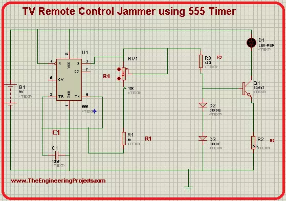
Hey pupils, welcome to The Engineering Projects. We hope you are doing great. In today's simulation in Proteus ISIS, we'll seek the knowledge of an interesting topic. We are going to design a Television remote jammer in Proteus. We all are familiar with the TV Remote controller device and know it works when a light signal emitted by it is sensed by the television. Have a glance at the topics we will see in detail today:

  1. Introduction to 555 Timer TV Remote Control Jammer.
  2. Components of the circuit.
  3. Working principle of 555 Timer Jammer.
  4. Simulation of the Jammer of TV Remote Control using 555 Timer.

Moreover, you will also learn some interesting facts about the topic in DID YOU KNOW sections. let's jump to our first topic.

555 Timer TV Remote Control Jammer

Remote controls do not require any introduction. We all use many types of remote controller devices in our daily lives. The TV Remote controls work on the principle of Infrared light. Yet, what if we do not want to give any access to other users or there is a requirement of blocking the signals from the remote controller device. In this case, jammers are useful because they do not alter any functioning of remote controls and just distract the television to sense the light signals. On this basis, we define the 555 Timer TV Remote Control Jammer as:

  • The 555 Timer TV Remote Jammer is a device used to jam the Infrared Lights emitted by the remote control, by producing a constant pulse of signals and distract the remote controller signals.

Before starting the working of the TV Remote control Jammer, let's have a piece of quick information on how does the TV Remote works. When we press the button of the remote, it sequentially emits the pulses. These pulses are then received by the IR Reciever present in the Television. Each time, every button has its own frequency of pulses so that the IR Reciever can sense which button is pressed. Then the TV act according to our command.

Now, in the case, when we want to cease the television to sense these signals, we just create a pulse, more powerful than TV remote controller, to disturb the pulse from the TV remote controller, so that the TV will not be able to sense pulses from TV Remote. We'll find how does this works in a bit.

DID YOU KNOW?
  • In electronics, the Jammer is any device that is used to prevent the instruments to sense the signals, waves or other mediums to cease their response.

Components used in TV Remote Jammer

In our circuit, we are going to use different components such as diodes, resistors, capacitors, etc. Out of them, 555 Timers and transistors are important to understand.

555 Timer in TV Remote control Jammer

The 555 Timer is an excellent Integrated circuit used in thousands of electronic circuits. It is used to transmit the pulses and control the flow of the circuit. The main reason behind its large number of projects and circuits is its modes. Basically, the 555 Timer can be used in three modes:

  • Astable Mode
  • Bistable Mode
  • Monostable Mode

For our circuit, we'll go for Astable Multivariable mode. This mode is chosen so because the IR waves from the remote control have very specific wave frequencies. In this way, when the waves from TV control Jammer will be Astable, this will be better to distract the TV from the remote's pulses. The 555 Timers is an 8 pin IC. In our circuit, pin 5 and pin 7 of the 555 Timer will remain unconnected. Other pins will be connected according to their respected functions.

Transistor in Remote Control Jammer

It's an NPN Transistor with three terminals called Emitter, Collector, and Base Terminals. In our experiment, the BC547 transistor will be used. The transistor will act as an amplifier in the circuit to make the pulses generated by the 555 Timer more clear, strong, and effective.

Complete List of Components required

  1. 555 Timer IC
  2. Resistor
  3. Diode
  4. Capacitor
  5. POT HG
  6. LED
  7. Battery
  8. BC547
  9. Ground Terminal

Working of TV Remote Control Jammer using 555 Timer

  1. The working of the circuit starts when the 9V Battery starts its work.
  2. This power enters 555 Timer through its two pins. The 555 Timer, in our case, is in Astable mode.
  3. In this way, the 555 timer generates a pulse that is not stable.
  1. To make the pulses more strong and effective, we use the Transistor. The transistor here works as an amplifier and amplifies the pulses coming towards it through its base terminal.
  2. The output of 555 Timer IC then passes through a couple of Diodes that are connected to the base and Emitter terminal of the BC547.
  3. Ultimately, the pulses of the 555 Timer IC pass through the LED and then to the collector Terminal of the Transistor.
  4. The LED shows the speed of the output pulses.
  5. This abrupt pulse is enough to distract the Infrared Reciever of the Television.
  6. So, as a result, we get a strong pulse of 36KHz-38KHz carrier frequency,

TV Remote Jammer circuit using 555 timers in Proteus

The simulation of the circuit is easy if you follow the steps given below carefully. So Let's go ahead.

Procedure to design circuit of TV Remote Jammer

  • Excite you Proteus Software and start a new Project.
  • Hit the "P" button then choose the first 8 components from the window that appeared.
  • Now arrange all the chosen components on the screen by following the image given next.
  • Go to the left side of the screen>Termnals mode>Ground and attach this ground terminal below the circuit.
DID YOU KNOW?
  • The mode of 555 Timer is identified by the components and their manner of connection with 555 Timer.
  • You can change the frequency of the pulses by changing the values of the components.
  • This change can easily be detected by observing the speed of the power entering the LED.
  • To connect them, let's use connecting wires.
  • You can alter the values of some components as:
POT HG: 1K, R1: 1K, R2: 5.6, R3:470, C:110nF,Battery:9V.
  • Go to virtual instrument Mode>Oscilloscope and fix it with the LED's output.
  • Finally, at the present moment, we are going to simulate our circuit.
  • Click on the play button and set the values of voltage and frequency through nobs.
  • The output of the oscilloscope will show that waves are formed frequently.

In the end, we conclude that we can design the circuit of the TV remote control jammer using the 555 Timer in Proteus. We had a short introduction to how does TV Remote works, we saw how can we jam its signal, we found how does the circuit works and at the end, we design a full circuit of a TV remote control jammer with the help of 555 timers in Proteus ISIS. This circuit emits a constant bit of 1.775 meters per second and the frequency ranges from 36KHz to 38KHz.

Traffic Light Circuit using 555 Timer in Proteus

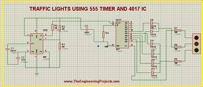
Hey pals! Welcome to the board. We are talking about a fascinating experiment about The Engineering Projects. We all know about the Traffic Lights. But today, we'll see inside the Traffic Lights and find some interesting working of the circuit of Traffic Lights. Before this, just have a look at the topics of discussion:

  1. What is the Traffic Lights circuit with 555 Timer?
  2. What does the 555 timer do in Traffic Lights?
  3. What is the purpose of the 4017 IC Counter in the circuit?
  4. How does the circuit of Traffic Lights work with 555 Timer IC?
  5. How can we perform experiments with the circuit of 555 Timer Traffic Lights in Proteus ISIS?

In addition, we'll see some important points about the topic in DID YOU KNOW sections.

Traffic Lights circuit with 555 Timer

Whenever we rush toward any road that has a heavy flow of vehicles, we always follow some traffic rules. One of the most fundamental traffic rules is to follow the traffic lights. These traffic lights direct the vehicles to start or stop moving at the road according to our turn. These turns are decided by the Traffic Lights. The traffic Lights show the different colored lights and these lights turn on and off in a sequence. We know all these things, but we are revising these to get the logic behind the scene. we define the Traffic Lights technically as:

"The traffic lights are the combination of three LEDs colored as red, amber and green that are connected in a specialized circuit that gives the output from the LEDs in a specific format and this format is used to control the flow of traffic."

These LEDs are enclosed in a metallic body. Traffic Light signals are so useful that 99% of the countries use them. This makes the circuit one of the most fundamental and common circuits to understand.

There are many devices through which the Traffic Lights may be controlled. Out of which, two are common:

  1. Traffic Lights with the D Flip Flop.
  2. Traffic Lights with 555 Timer

We have discussed the 1st method in our previous tutorial, Let's have a look at the next one.

555 Timer IC Performance in Traffic Lights

before starting the simulation, let's have a look at its components briefly. The circuit of Traffic Lights uses a very common yet powerful device i.e, 555 Timer IC. The 555 Timer is so useful that it is said that annually, a billion of 555 Timers are produced and it is considered as the most popular IC of the year 2017. We introduce the 555 Timer as:

"The 555 Timer is a common 8 pins Integrated Circuit used in a variety of oscillation generators and Timers to generate a pulse of the signals that control the output sequentially."

In our experiment, we'll apply the Mono-stable Multi-vibrator mode of the 555 timer. The output of 555 Timer in this mode is in the form of a single pulse of current that has a specific length. This pulse is sometimes called the one-shot pulse.

4017 IC in the 555 Timer Traffic Lights

The 4017 is the special IC that is usually coupled with the 555 Timer. It works on the pulse generated by the 555 Timer and the definition for the 4017 IC is given as:

  • "The 4017 is 16 pins counter and decoder of 555 Timer IC that generates a decade counter output from its output pins and the outputs advances from one to another with the positive edge of the clock pulse."

Once the clock pulse of 4017 IC in the traffic Lights goes from low to high, the IC started its cycle again and we get a sequential Logic output. The pins 3 to 12 of the 4017 IC Counter are said to be the output pins of the 4017 and we'll connect the traffic lights with them.

Working of Traffic Lights using 555 Timer IC

  1. The Working of the circuit starts with the power connected to the Vcc terminal of 555 Timer IC.
  2. the power in the 555 Timer in Mono-stable Multi-vibrator mode produces a uniform pulse of current that is stabilized with the help of capacitors used with the 555 Timer IC.
  3. The current is then fed into the clock terminal of the 4017 decade counter IC that decodes these pulses of 555 Timer IC and produces the stream of output at its output terminals.
  4. The terminals of the 4017 IC are connected to the diodes in a specific manner. These diodes conduct the electricity on only one side and so that a specialized sequence of the current is found at the outputs of these diodes.
  5. There are two sets of the diode connections. Four diodes are connected in a set and two in another. The output of 1st set is fed to Green Light of the Traffic Lights. The Amber and Red lights of the circuit are connected with the second set.
  6. The output of these two sets is connected with the resistor and then finally this current passes to the traffic Lights signal.
  7. In the end, we get a specialized, clear and automatic output from the traffic lights.

Simulation of the circuit of 555 Timer Traffic Lights in Proteus ISIS

At the moment, we are going to design the circuit of the experiments. So let's start.

Devices required for 555 Timer Traffic Lights

  1. 555 Timer IC
  2. 4017 IC
  3. Capacitors - 3
  4. Resistors - 7
  5. Diodes - 6
  6. Traffic lights
  • Fire up your Proteus Software.
  • Choose the material from pick Library through "P" button.
Let's divide the circuit design into three parts:
  1. 555 Timer connections
  2. 4017 IC Counter connections
  3. Connection of 555 Timer and 4017 IC

555 Timer Connections

  • Choose the 555 Timer from the component's area and arrange it on the left side working area.
  • Select the resistor then  arrange three resistors with pin 3, 6 and 7.
  • Take capacitor and set two capacitors with pin 2 and 5 of 555 Timer.
  • Go to terminal mode and set a Ground terminal at the Ground pin of the 555 Timer.
  • Connect all the components of 555 Timer IC as:

Connections of 4017 IC

  • Go to components, choose 4017 IC.
  • Select diode and arrange the 7 diodes with the output pins on the right side of 4017 IC.
  • Take care with the direction of the diodes.
  • Set a resistor between the pins 13 and 16 of 4017 IC.
  • Arrange three resistors  just after the diodes.
  • Now set a Traffic Light signal on the right side of the resistors.

DID YOU KNOW?????????????????????????????

It is said by AAA, the average American spends 58.6 hours every year waiting at the red light of traffic signal.
  • The circuit now looks like the image given next:

Connection of ICs

  • Now, at the moment, we'll connect the ICs to finally set our circuit.
  • Set a capacitor between both these ICs.
  • Alter the names of the components by given them numbering so that Proteus may distinguish between different Resistors, Capacitors, diodes and ICs.
  • Change the values of each component according to the table given next:
Component Values
C1 0.01uF
C2 47uF
C3 6.8nF
R1 23k ohm
R2 10k ohm
R3 22K ohm
R4 100k ohm
R5 100 ohm
R6 100 ohm
  • Observe deeply the image given below and connect all the components with the help of connecting wires.
  • Our circuit is now good to go, Let's tap the play button and simulate the circuit.
The circuit shows the required output well. If you found any error, look at the steps given above again.

DID YOU KNOW????????????????

The working speed of the Traffic Lights can be varied by changing the values of capacitors connected with  pin 5 and 2 of the 555 Timer IC.
So, today we saw a fantastic circuit in which we learned that what are the Traffic lights signal using 555 timer, how does the ICs of 555 timer and 4017 IC Counter work with each other to show the output of the Traffic Lights and we designed the circuit of 555 Timer Traffic Lights in Proteus ISIS. If you have any questions, you can contact us through the comment sections.
Syed Zain Nasir

I am Syed Zain Nasir, the founder of <a href=https://www.TheEngineeringProjects.com/>The Engineering Projects</a> (TEP). I am a programmer since 2009 before that I just search things, make small projects and now I am sharing my knowledge through this platform.I also work as a freelancer and did many projects related to programming and electrical circuitry. <a href=https://plus.google.com/+SyedZainNasir/>My Google Profile+</a>

Share
Published by
Syed Zain Nasir