Hi Friends! Hope you’re well today. Happy to see you around. In this post, I’ll walk you through How to Install PCBWay Plugin for KiCAD PCB Software.
Before we move further, let’s get a brief overview of KiCAD PCB Software.
KiCAD is a free and open-source electronic design application mainly developed to draw schematics and PCB layouts. It is open-source which means anyone can use it to develop and modify electronic designs. The tool can effortlessly run on Windows, macOS and Linux. The main window of the application comes with 8 different software tools used to make PCB layouts and schematics.
Hope you’ve got a sneak peek at the software. Now we’ll get to know how to install the PCBWay Plugin for KiCAD.
How to install PCBWay Plugin for KiCAD PCB Software?
When you install ...
Matrices are an essential topic in different fields of study, especially in mathematics, where you have a bulk of data and want to organize, relate, transfer, and perform different operations on data in a better manner. We have studied a lot of types and operations on the matrices and have worked on different types with the help of MATLAB. Today, we are here to present the applications of the matrices in different fields of study to clarify the importance of this topic. So, have a look at the list of topics we are going to learn. Yet, first of all, I am going to describe what a matrix is.
What is a Matrix?
In the fields of physics and mathematics, there is the use of different types of numbers in groups of various types. In order to organize the data into a manageable format, matrices ar ...
Hey students welcome to another tutorial in The Engineering Projects where we are going to learn a lot about matrices. If you are a beginner to the metrics, then you should go to learn the fundamentals of matrices. Yet, if you know the basic introduction, you are at the right lecture because we are learning about the special kinds of matrices and you are also going to see the matrices in action using MATLAB. So, here is a simple list of today’s topics.
What is a matrix?
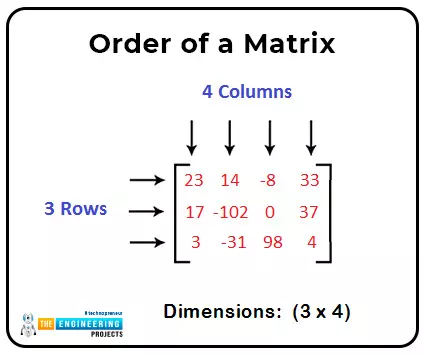
How can we identify the matrix with the help of its general form?
What are the different types of matrices?
What is the concept of transpose while dealing with matrices?
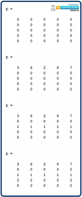
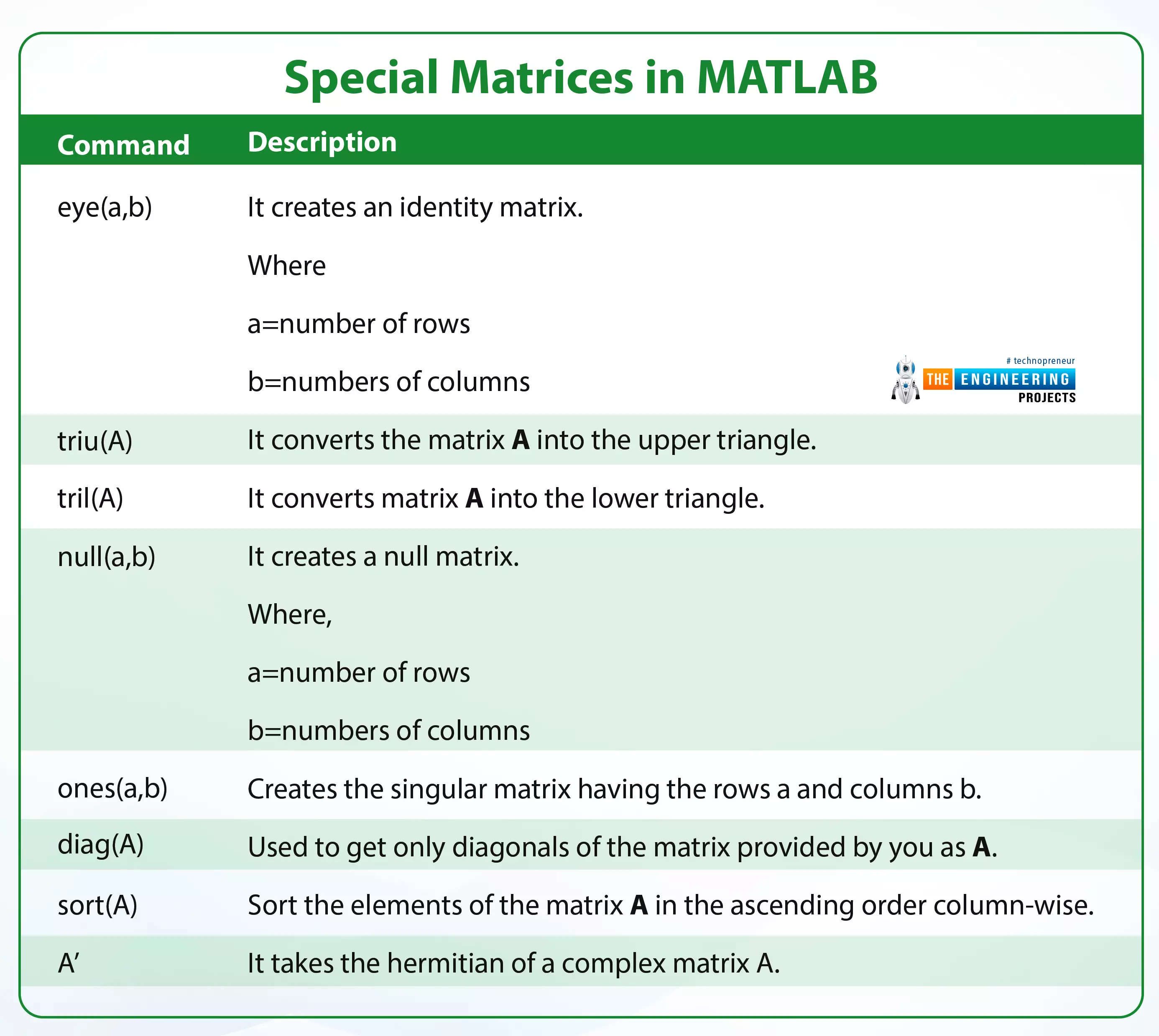
How can we implement these types of matrices in MATLAB by different commands?
What is a Matrix?
A matrix is a type of array that stores da ...
Hello, learners welcome to The Engineering Projects. We are working on MATLAB, and in this tutorial, you are going to learn a lot about matrices in MATLAB. We are going to learn them from scratch, but we will avoid unnecessary details about the topic. So, without wasting time, have a look at the topics that you will learn in detail.
What is an array?
What is the matrix?
How can we declare a matrix in MATLAB?
What are the different types of matrices?
Can we find the unknown values of two equal matrices?
How can we solve the simultaneous equation in MATLAB?
What is an Array?
In this world of technology, the use of data is everywhere, and therefore, we can say there is a need for arrays in every field. You will find the reason soon. But before this, look at the introduction of a ...
Hello readers, Welcome to another tutorial about the signal and system. In this lecture, you are going to read details about the ramp response of a signal. In the past lectures, we have been dealing with different types of responses of LTI systems, and therefore, we know that linear invariant systems, or LTI systems, are those which follow the rules of linearity and are also time-invariant. So, at present, our focus is to examine what happens when the ramp signals are fed into the LTI system and which type of output signal we receive. Here is a glimpse at today’s topic that we will learn deeply.
What is the RAMP signal?
How can you define the ramp response?
How to use the ramp function in MATLAB to get the ramp response?
What are some important properties of the ramp function?
How i ...
Hello learners, Welcome to another tutorial on signals and systems. We are learning about the responses of the signals. We all have experience in situations where the change in the frequency of a system, such as radios or control systems, results in a change in the working or result of that system. So we have the idea that frequencies play an important role in different types of systems. In the previous lecture, we saw the impulse response of the system. Our mission today is to learn about the frequency response of the LTI system. We will learn all the basic information about the topic and will revise some important points as well. To do this, have a look at today’s concepts:
What is the LTI system?
What is frequency response?
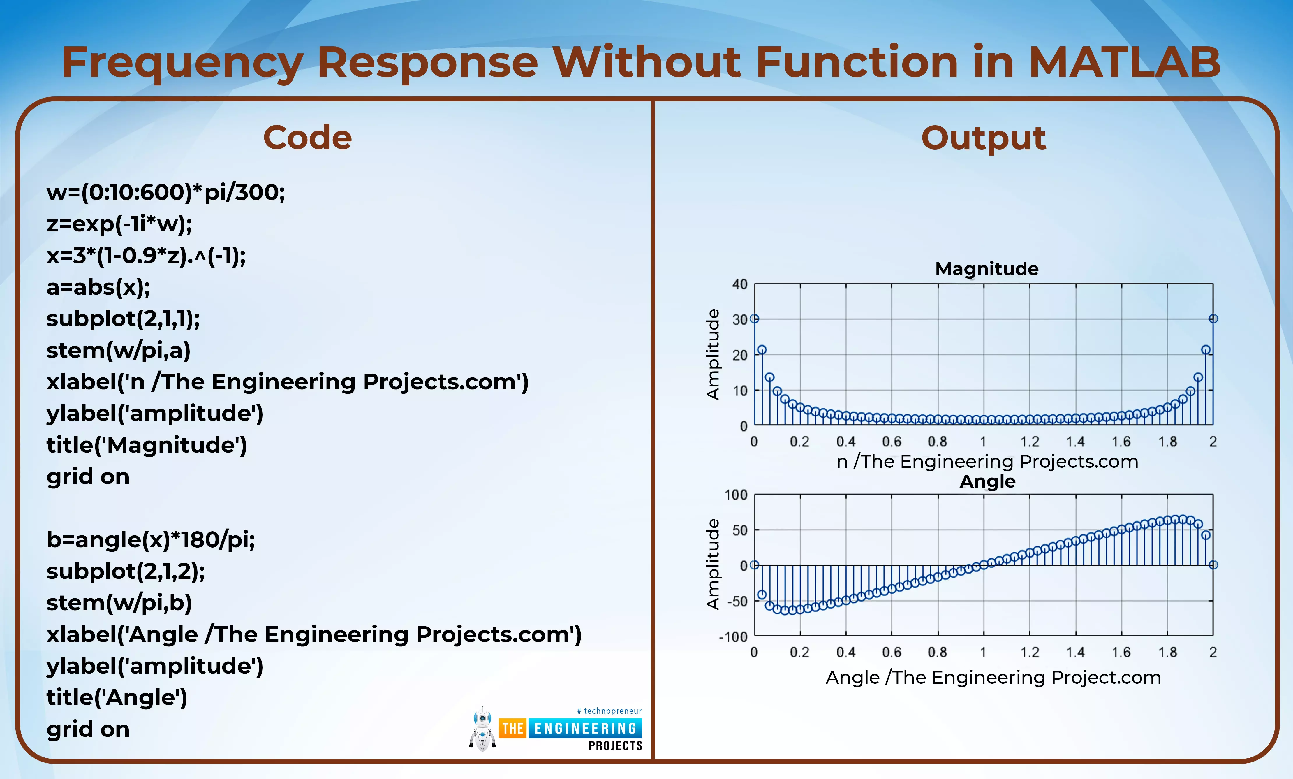
How is frequency response performed without the function i ...
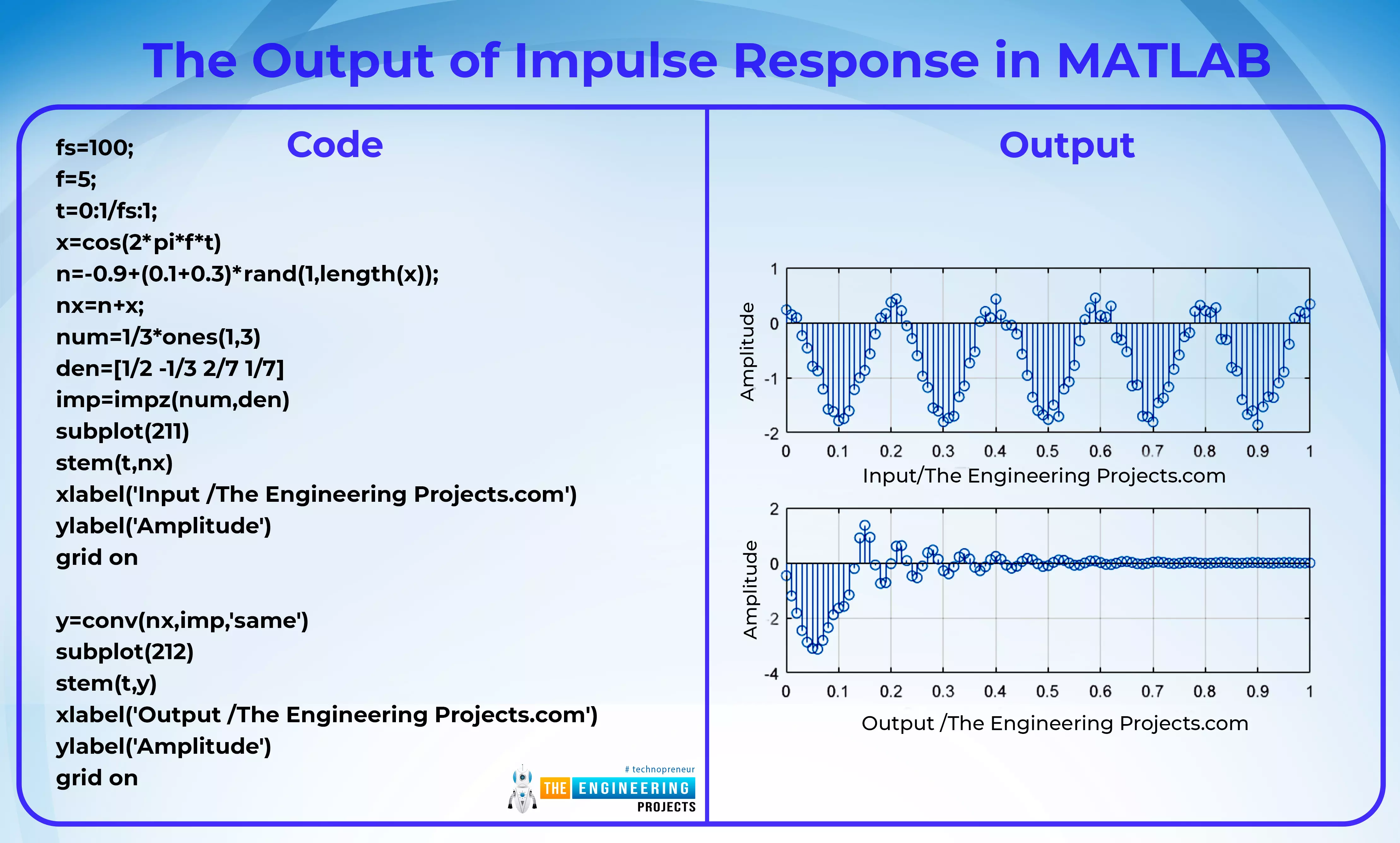
Hello learners, welcome to another topic of signals and systems. We hope you are having a reproductive day and to add more information in the simplest way to your day, we are discussing the responses in discrete-time signals. If you do not get the idea of the topic at the moment, do not worry because we are going to learn it in detail and you are going to enjoy it because we are making interesting patterns in MATLAB as the practical implementation of the topics. Have a look at the points that we are making clear today.
What is the LTI system?
What is impulse response?
How can we get the impulse response in MATLAB?
How can we have the output signal using codes and impulse response in MATLAB?
As we have learned so far in this series, there are two types of signals based on the ...
Hey, pupils welcome to the next session about the Fourier transform. Till now, we have learned about the basics of Fourier transform. It is always better to understand all the properties of a mathematical tool to understand its workings and characteristics. You will observe that most of its properties are similar to the topics that we have discussed before, and the reason is, that all of them are transforms, and the core objective of these transforms is the same. We have learned about the simple and easy discussion of the Fourier Transform, but when dealing with complex problems, it involves the usage of different properties so that we do not have to repeat the calculations all the time to get the required results. Have a look at what you are going to learn today:
What are the basic prope ...
Hi Guys! Hope you’re well today. I welcome you on board. In this post, I’ll walk you through How to Install PCBWay Plugin for FreeCAD PCB Software.
Before we move further and help you with the installation of the plugin, let’s get a brief introduction to the FreeCAD software.
FreeCAD is a free and open-source parametric 3D modeler used to design real-life objects. With parametric modeling, you can easily modify your design and change its parameters. The tool is mainly used in mechanical engineering for product design and also proves to be handy in electrical engineering for electronic board designs. It supports Windows, Linux and macOS operating systems. Python programming language is primarily used to extend the overall functioning of the software.
Hope you’ve got an ...
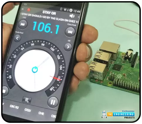
Throughout our lives, we've relied on Radio and tv stations to keep us engaged. While we're on the subject of contradictions, it's also fair to say that these Stations can become tedious at times due to the RJ rambling on about nothing or annoying advertisements, and this may have left you wondering why you can't own a Radio station to broadcast your data over short distances.
Almost any electronics technician uses coils and other hardware to make an FM transmitter, although the tuning process is time-consuming and difficult. Setting up your FM station and going live in your neighborhood shouldn't take more than 30 minutes using an RPi. If you use the right antenna, you must be able to transmit to your school or community within 50 meters. Wow, th ...