How to Properly Dispose of Solar Batteries: Everything You Need to Know

So you've installed a beautiful new solar energy system around your house or property. You're saving tons on your electric bill and never have to worry about blackouts, power surges, or planned outages—you control your power source now. Here's the problem: What do you do when you need to dispose of everything?

Eventually, you will need to replace the solar panels and the solar battery, which powers the whole system. Disposing of solar batteries isn't exactly simple, and it needs to be handled with the utmost care. But it is easy to navigate if you know the proper steps to take—and what to avoid. Here's our complete guide.

Disposing of the Battery

If you've recently purchased a solar energy system or portable solar generator, you know the current solar battery price . It's not low, but it has improved in recent years as technology evolves. Lithium batteries are rechargeable, but they don't last forever. 

Once your lithium battery dies or needs to be replaced, you should first call your local waste management authority. They will be able to direct you to the proper place to dispose of your solar battery safely.

Inquire About Recycling Alternatives

The lithium batteries often used for solar generators contain tons of materials that would adversely impact the environment if they were left to decompose in landfills. The National Library of Medicine warns about metals such as copper, nickel, and lead. Other concerning components include toxic and flammable organic chemicals that contain compounds like LiClO4, LiBF4, and LiPF6.

For this reason, you should ask the waste management authority about recycling options. Those chemicals must be disposed of properly, and many metals can be used elsewhere in other construction and manufacturing projects.

What Can Be Recycled?

Metals currently comprise about 13% of all that is thrown into the recycling . Still, if people took the time to learn how to recycle complicated objects such as lithium batteries, that number could rise even higher. Plenty of the materials used to make lithium batteries for solar generators can be recycled. Those that can be reused include:

  • Glass, which is the primary material used in the manufacturing of photovoltaic panels and can be found inside lithium batteries

  • Aluminum, which is 100% recyclable

  • Copper, nickel, and lead are all largely recyclable, and copper can be 100% recycled and reused.

Knowing what you can recycle is the first step to figuring out how to recycle it properly. 

The Cost of Not Recycling

As landfills rise, the cost to our environment grows. When items like lithium batteries containing dangerous compounds are thrown into landfills, they can decompose, and those compounds can render everything they touch toxic. 

The dangers of landfills include destroying natural animal habitats, producing toxic methane gas, contaminating water supplies, the production of ammonia, and more. Make sure to dispose of your battery safely.

Making the Smart Choice

You can make money from recycling your lithium battery, and you'll be helping save the environment in the process. There's no reason not to follow these steps.

Interface 7-Segment Display with Raspberry Pi 4

Thank you for being here for today's tutorial of our in-depth Raspberry Pi programming tutorial. The previous tutorial taught us how to install a PIR sensor on a Raspberry Pi 4 to create a motion detector. However, this tutorial will teach you how to connect a single seven-segment display to a Raspberry Pi 4. In the following sections, we will show you how to connect a Raspberry Pi to a 4-digit Seven-Segment Display Module so that the time can be shown on it.

Seven-segment displays are a simple type of Display that use eight light-emitting diodes to show off decimal numbers. It's common to find it in gadgets like digital clocks, calculators, and electronic meters that show numbers. Raspberry Pi, built around an ARM chip, is widely acknowledged as an excellent Development Platform. Its strong processing power can do amazing things in the hands of electronics enthusiasts and students. If we can figure out how to have it talk to the outside world and process data via an output, then we'll have a real chance of accomplishing all this. We analyze the data by viewing it on an LCD screen or other Display. Numerous sensors can detect specific parameters in the physical world and convert them to the digital world. It would never make sense to utilize a PI LCD panel to display a minimal quantity of information. Here, a 7-Segment or 16x2-Alphanumeric LCD panel is the preferred method of presentation.

There are few uses for a 7-segment display that don't need an LCD panel, even though a 16x2 LCD is preferable in most. If all you need to do is show some numbers, then an LCD, which has the downside of having a small character size, is excessive. Compared to a regular LCD screen, seven segments have the upper hand in dim environments and can be seen from wider angles. Let's get started.

Where To Buy?
No.ComponentsDistributorLink To Buy
1BreadboardAmazonBuy Now
2Jumper WiresAmazonBuy Now
3Raspberry Pi 4AmazonBuy Now

Components

  • Jumper wires

  • Seven segment display

  • 1KΩresistors

  • Breadboard

The 7-Segment and 4-Digit Display Modules

The seven segments of a 7 Segment Display are each lit up by an individual LED to show the digits. To show the number 5, for example, you would make the glow pins for segments a, f, g, c, and d on the 7-segment high. This particular 7-segment display is a Common Cathode version, although there is also a Common Anode version.

One 7-Segment Display Interfacing with Pi 4

The wiring diagram for connecting a 7-segment display to a Raspberry Pi is shown below. Here, 7-Segment Common Cathode has been utilized.

So, we'll simulate an 8-bit PORT on PI using its eight GPIO pins. Here, GPIO12 is the Most Significant Bit (MSB), while GPIO13 is the Least Significant Bit (LSB) (Most Significant Bit).

If we wish to show the number 1, we must activate both segments B and C. We must supply voltage to GPIO6 and GPIO16 to power segments B and C. Accordingly, the hexadecimal value of "PORT" is "06," and the byte value of "PORT" is "0b00000110." If we raise both pins to their highest positions, the number "1" will be shown.

The value for every displayable digit has been recorded and saved in a Character String with the label 'DISPLAY .'We have then used the Function 'PORT' to call those values one at a time and display the relevant digit.

Explanation of the Code

Once everything is wired up according to the schematic, we can power up the PI and begin using PYTHON to write the program. Below is a function that allows us to program the GPIO pins on the PI, and we'll go over the few commands we'll be using in the PYTHON program to do so. We are also changing the name of the GPIO pins in the hardware from "GPIO" to "IO," which will be used throughout the code.

import RPi.GPIO as IO

The general-purpose input/output (GPIO) pins we need to use may be occupied with other tasks. If that's the case, the program's execution will be interrupted by warnings. The below command instructs the PI to continue running the software regardless of the warnings.

IO.setwarnings(False)

Pin numbers on the board and pin functions can be used to refer to PI's GPIOs. This GPIO5 is similar to the one labeled "PIN 29" on the board. Here we specify whether the number 29 or the number 5 will stand in for the pin.

IO.setmode (IO.BCM)

To use the LCD's data and control pins, we have assigned those functions to eight of the GPIO pins.

IO.setup(13,IO.OUT)

IO.setup(6,IO.OUT)

IO.setup(16,IO.OUT)

IO.setup(20,IO.OUT)

IO.setup(21,IO.OUT)

IO.setup(19,IO.OUT)

IO.setup(26,IO.OUT)

IO.setup(12,IO.OUT)

If the condition between the brackets evaluates to true, the looped statements will be run once. The value of PIN13 would be HIGH if and only if bit0 of the 8-bit 'pin' is true. There are eight 'if else' conditions, one for each of bits 0 through 7, so that each LED in the seven-segment Display can be set to either the High or Low state, depending on the value of the corresponding bit.

if(pin&0x01 == 0x01):

   IO.output(13,1)

else:

   IO.output(13,0)

As x increases from 0 to 9, the loop will be run 10 times for each command.

for x in range(10):

The following command can create an infinite loop, with which the statements included within the loop will be run repeatedly.

While 1:

All other commands and functions have been commented on in the following code.

Single 7-segment Display complete code

import RPi.GPIO as IO            # calling for the header file, which helps us use GPIO's of PI

import time                              # calling for time to provide delays in the program

DISPLAY = [0x3F,0x06,0x5B,0x4F,0x66,0x6D,0x7D,0x07,0x7F,0x67]            # string of characters storing PORT values for each digit.

IO.setwarnings(False)            # do not show any warnings.

IO.setmode (IO.BCM)           # programming the GPIO by BCM pin numbers. (like PIN29 as‘GPIO5’)

IO.setup(13,IO.OUT)             # initialize GPIO Pins as outputs

IO.setup(6,IO.OUT)

IO.setup(16,IO.OUT)

IO.setup(20,IO.OUT)

IO.setup(21,IO.OUT)

IO.setup(19,IO.OUT)

IO.setup(26,IO.OUT)

IO.setup(12,IO.OUT)

def PORT(pin):                    # assigning GPIO logic by taking the 'pin' value

    if(pin&0x01 == 0x01):

        IO.output(13,1)            # if  bit0 of 8bit 'pin' is true, pull PIN13 high

    else:

        IO.output(13,0)            # if  bit0 of 8bit 'pin' is false, pull PIN13 low

    if(pin&0x02 == 0x02):

        IO.output(6,1)             # if  bit1 of 8bit 'pin' is true, pull PIN6 high

    else:

        IO.output(6,0)            #if  bit1 of 8bit 'pin' is false, pull PIN6 low

    if(pin&0x04 == 0x04):

        IO.output(16,1)

    else:

        IO.output(16,0)

    if(pin&0x08 == 0x08):

        IO.output(20,1)

    else:

        IO.output(20,0)   

    if(pin&0x10 == 0x10):

        IO.output(21,1)

    else:

        IO.output(21,0)

    if(pin&0x20 == 0x20):

        IO.output(19,1)

    else:

        IO.output(19,0)

    if(pin&0x40 == 0x40):

        IO.output(26,1)

    else:

        IO.output(26,0)

    if(pin&0x80 == 0x80):

        IO.output(12,1)            # if  bit7 of 8bit 'pin' is true, pull PIN12 high

    else:

        IO.output(12,0)            # if  bit7 of 8bit 'pin' is false, pull PIN12 low

While 1:

    for x in range(10):            # execute the loop ten times incrementing x value from zero to nine

        pin = DISPLAY[x]        # assigning value to 'pin' for each digit

        PORT(pin);                  # showing each digit on display 

        time.sleep(1)

Output

The process of displaying a single number character on a 7-segment display is complete. However, we'd need more than a single 7-segment display to express information with more than one digit. Therefore, we will use a 4-digit seven-segment display circuit for this session.

Four individual Seven-Segment Displays have been linked up here. For a 4-digit 7-segment display, we know that each module will have 10 pins, so there will be 40 pins total. Soldering that many pins onto a dot board would be a hassle for anyone; thus, I recommend that anyone using a 7-segment display do so by purchasing a module or creating their PCB. See below for a diagram of the relevant connections:

In the preceding diagrams, we can see that the A-lines of all four displays are linked together as one A, and the same is true for B, C.... up until DP, which is essential for understanding how the 4-digit seven-segment module functions. Put another way, if trigger A is activated, the state of all 4 A's should be high.

Nonetheless, this never occurs. The four extra pins labeled D0 through D3 (D0, D1, D2, and D3) let us select which of the four displays is driven high. As an illustration, if I want my output to appear solely on the second Display, I would set D1 to high and leave D0, D2, and D3 at low. Using pins D0–D3 and A–DP, we can easily choose which displays should be on and which characters should be shown.

Using a Pi 4  to interface with a 4-digit, 7-segment display module

Let's check the many options for interfacing this 4-digit seven-segment Display with the Raspberry Pi. As can be seen in the diagram below, there are 16 pins on the 7-segment module. Even if your module's resources are limited, it will provide at least the following.

  • Segmented pins, either 7 or 8 segments (pins 1 to 8)

  • Pin holder to the ground (here pin 11)

  • A 4-digit code to unlock the door (pins 13 to 16)

See below for the wiring diagram of a digital clock built with a Raspberry Pi and a 4-digit Seven-segment display module:

You can also use the following table to ensure your connections are correct and follow the diagrams.

Locating the module's pins is the first step in making electrical connections. Identifying the Raspberry Pi's GPIO pins can be tricky; I've included an image to help.

Raspberry Pi programming

Here, RPi is programmed in the Python programming language. The Raspberry Pi can be programmed in a wide variety of ways. Since Python 3 has become the de facto standard, we've opted to use that version as our integrated development environment (IDE). At the bottom of this guide, you'll find the whole Python code.

We'll go over the PYTHON instructions we'll be using for this project: first, we'll import the library's GPIO file; next, using the below function, we'll be able to program the Pi 4's GPIO pins. We are also changing the name of the GPIO pins in the hardware from "GPIO" to "IO," which will be used throughout the code. We've brought in time and DateTime to get the current time from Rasp Pi.

import RPi.GPIO as GPIO

import time, DateTime

The GPIO pins we're trying to use are already being used for something else. The program's execution will be interrupted with warnings if this is the case. The PI will be instructed to disregard the errors and continue with the software using the below command.

IO.setwarnings(False)

The physical pin number and the corresponding function number can refer to PI's GPIOs. As with 'PIN 29,' GPIO5 is a physical component on the circuit board. In this case, we specify whether the number "29" or "5" will stand in for the pin. GPIO. In BCM notation, GPIO5 pin 29 will be represented by a 5.

IO.setmode (GPIO.BCM)

As is customary, we'll start by setting the pins to their default values; in this case, both the segment and digit pins will be used as outputs. In our code, we organize the segment pins into arrays and set their values to zero by declaring them to be GPIO.OUT.

segment8 = (26,19,13,6,5,11,9,10)

for segment in segment8:

    GPIO.setup(segment, GPIO.OUT)

    GPIO.output(segment, 0)

We do the same thing with the digital pins, but we set them to output and set them to zero by default.

#Digit 1

    GPIO.setup(7, GPIO.OUT)

    GPIO.output(7, 0) #Off initially

    #Digit 2

    GPIO.setup(8, GPIO.OUT)

    GPIO.output(8, 0) #Off initially

    #Digit 3

    GPIO.setup(25, GPIO.OUT)

    GPIO.output(25, 0) #Off initially

    #Digit 4

    GPIO.setup(24, GPIO.OUT)

    GPIO.output(24, 0) #Off initially

Numbers on a seven-segment display must be formed into arrays. To show a single digit, we need to toggle the on/off status of all but the dot pin of the 7-segment Display. For the numeral 5, for instance, we can use this setup:

For all alphabets and numerals, there is an equivalent sequence number. You can write on your own or utilize the handy table provided.

Using this information, we can create arrays for each digit in our Python code, as demonstrated below.

null = [0,0,0,0,0,0,0]

zero = [1,1,1,1,1,1,0]

one = [0,1,1,0,0,0,0]

two = [1,1,0,1,1,0,1]

three = [1,1,1,1,0,0,1]

four = [0,1,1,0,0,1,1]

five = [1,0,1,1,0,1,1]

six = [1,0,1,1,1,1,1]

seven = [1,1,1,0,0,0,0]

eight = [1,1,1,1,1,1,1]

nine = [1,1,1,1,0,1,1]

Let's bypass the function in the code that would otherwise be executed before entering the while loop and begin displaying characters on our 7-segment Display. If you hook up a Raspberry Pi to the internet, it will read the current time and divide it into four separate variables. For instance, when the time is 10.45, the values assigned to h1 and h2 will be 1 and 0, while m1 and m2 will be 4 and 5, respectively.

now = DateTime.DateTime.now()

    hour = now.hour

    minute = now.minute

    h1 = hour/10

    h2 = hour % 10

    m1 = minute /10

    m2 = minute % 10

    print (h1,h2,m1,m2)

These four numbers will be displayed on one of our four digits. The lines below can be used to convert a variable's value to a decimal. Here, we show the value in variables on the 7-segment Display by using the function print segment (variable) with the digit 1 set to the highest possible value. You may be asking why we turn off this digit and why there's a delay after that.

GPIO.output(7, 1) #Turn on Digit One

print_segment (h1) #Print h1 on segment

time.sleep(delay_time)

GPIO.output(7, 0) #Turn off Digit One

This is because the user will only be able to see the full four-digit number if all four digits are shown at once, and we all know that this isn't possible.

How, then, can we simultaneously show all four digits? With luck, our MPU is considerably quicker than the human eye. Therefore we offer one number at a time but exceptionally quickly. The MPU and segment display are given 2ms (variable delay time) to process each digit before we go on to the next. A human being cannot detect this 2ms lag; therefore, it appears as though all four digits illuminate simultaneously.

Understanding how to use print segment(variable) is the final puzzle piece. Arrays that have been declared outside of this function are used within it. As a result, the value of any variable passed to this function must be inside the range (0-9) so that the character variable can use in a meaningful comparison. Here, we check the variable against the value 1. The same is true for all comparisons with numbers between zero and nine. Assigning each value from the arrays to the appropriate segment pins is what we do if a match is found.

def print_segment(character):

    if character == 1:

        for i in range(7):

            GPIO.output(segment8[i], one[i])

Show the time on a 4-digit 7-segment display.

Use the provided schematic and code to connect your components and set up your Raspberry Pi. Once you've finished setting everything up, you can open the software and check the 7-segment Display to see the time. However, before doing this, you should check a few things.

  • If you want to be sure your Raspberry Pi isn't stuck in the past, you should update its time.

  • If you want to utilize a 7-segment display on your Raspberry Pi, you'll need to plug it into an adapter rather than a computer's USB connection because of the large amount of current it consumes.

Complete code

import RPi.GPIO as GPIO

import time, DateTime

now = datetime.datetime.now()

GPIO.setmode(GPIO.BCM)

GPIO.setwarnings(False)

 #GPIO ports for the 7seg pins

segment8 =  (26,19,13,6,5,11,9,10)

for segment in segment8:

    GPIO.setup(segment, GPIO.OUT)

    GPIO.output(segment, 0)

    #Digit 1

    GPIO.setup(7, GPIO.OUT)

    GPIO.output(7, 0) #Off initially

    #Digit 2

    GPIO.setup(8, GPIO.OUT)

    GPIO.output(8, 0) #Off initially

    #Digit 3

    GPIO.setup(25, GPIO.OUT)

    GPIO.output(25, 0) #Off initially

    #Digit 4

    GPIO.setup(24, GPIO.OUT)

    GPIO.output(24, 0) #Off initially

null = [0,0,0,0,0,0,0]

zero = [1,1,1,1,1,1,0]

one = [0,1,1,0,0,0,0]

two = [1,1,0,1,1,0,1]

three = [1,1,1,1,0,0,1]

four = [0,1,1,0,0,1,1]

five = [1,0,1,1,0,1,1]

six = [1,0,1,1,1,1,1]

seven = [1,1,1,0,0,0,0]

eight = [1,1,1,1,1,1,1]

nine = [1,1,1,1,0,1,1]

def print_segment(charector):

    if charector == 1:

        for i in range(7):

            GPIO.output(segment8[i], one[i])

    if charector == 2:

        for i in range(7):

            GPIO.output(segment8[i], two[i])

    if charector == 3:

        for i in range(7):

            GPIO.output(segment8[i], three[i])

    if charector == 4:

        for i in range(7):

            GPIO.output(segment8[i], four[i])

    if charector == 5:

        for i in range(7):

            GPIO.output(segment8[i], five[i])

    if charector == 6:

        for i in range(7):

            GPIO.output(segment8[i], six[i])

    if charector == 7:

        for i in range(7):

            GPIO.output(segment8[i], seven[i])

    if charector == 8:

        for i in range(7):

            GPIO.output(segment8[i], eight[i])

    if charector == 9:

        for i in range(7):

            GPIO.output(segment8[i], nine[i])

    if charector == 0:

        for i in range(7):

            GPIO.output(segment8[i], zero[i])               

    return;

while 1:

    now = DateTime.DateTime.now()

    hour = now.hour

    minute = now.minute

    h1 = hour/10

    h2 = hour % 10

    m1 = minute /10

    m2 = minute % 10

    print (h1,h2,m1,m2)

    delay_time = 0.001 #delay to create the virtual effect

    GPIO.output(7, 1) #Turn on Digit One

    print_segment (h1) #Print h1 on segment

    time.sleep(delay_time)

    GPIO.output(7, 0) #Turn off Digit One

    GPIO.output(8, 1) #Turn on Digit One

    print_segment (h2) #Print h1 on segment

    GPIO.output(10, 1) #Display point On

    time.sleep(delay_time)

    GPIO.output(10, 0) #Display point Off

    GPIO.output(8, 0) #Turn off Digit One

    GPIO.output(25, 1) #Turn on Digit One

    print_segment (m1) #Print h1 on segment

    time.sleep(delay_time)

    GPIO.output(25, 0) #Turn off Digit One

    GPIO.output(24, 1) #Turn on Digit One

    print_segment (m2) #Print h1 on segment

    time.sleep(delay_time)

    GPIO.output(24, 0) #Turn off Digit One

    #time.sleep(1)

Output

A similar section should appear below if everything is functioning as it should.

7-segment Display limitations

Typically, only 16 hexadecimal digits can be shown on a seven-segment display. Some show the digits 0-9, whereas others can show more. Seven-segment displays can only show a maximum of 16 values due to a lack of input leads. However, LED technology does allow for more than this. Even with the help of integrated circuit technology, the possible permutations of the seven parts on the screen are very few.

Conclusion

This guide taught us how to connect a 7-segment screen to a Raspberry Pi 4. The seven-segment Display, which we learned is employed in digital timers, clocks, and other electrical gadgets, are a cheap, basic electrical circuit and reliable module. Seven-segment displays can either be "common-anode" (where the common point is the power input) or "common-cathode" (where the common end is grounded). After that, we coded some python scripts to show numbers on a single seven-segment model and the time across four such screens. Next, we'll see how to use a Raspberry Pi 4 as the basis for a low-power Bitcoin miner.

Advance Counter Functions in PLC Ladder Logic

Hi, my friends. Welcome to share a new tutorial in our ladder logic programming series. Today we will discuss counters in ladder logic programming using an expert’s view. So let’s wear the glasses of an expert in ladder logic programming and look deeply into counters, the types of counters, their variables and bits. In addition, techniques of using counters to solve a different kinds of problems that need counting. And without questions like every time, we will enjoy practicing programming and simulating all about counters. So with no further delay, let’s jump into our tutorial and nail that counters.

Counters in real life

Tell me, guys, if you can imagine an industrial project or machine that does not need to count parts, products, or processing cycles. Actually, in most cases in industry and practical operations, you will find counters everywhere you visit production lines or operating machines. So now, what are the types of counters and what is inside or belongs to counters, their variables and bits? Also, what are the techniques for utilizing counters in ladder logic programming?

Counter Types

As regards functionality, counters can be divided into count up and count down, as shown in figure 1. Counter-up and down instruction blocks are shown in CTU and CTD. One is to count up, and the other is used to count down. They are different in functionality. However, they have the same variables, parameters, and data bits. So let’s discuss all this data belonging to counters.

Counter data bits

Figure 2 images the data of counters. On the left tree, you guys notice the counters in the data files and on the right, see many counters that you can use in your ladder logic program. Also, the main variables are the preset value and the accumulator value by which you tell the program the counter will count up or down to what value. Also, you should know the left side of the rung is the input to the counter to activate it and let it counts when the input is high. While the right side is the output data bit of the counter which is the enable EN bit that tells the counter block has run okay. And the done bit DN that informs the counter reached the desired preset value by turning into high when the accumulator variable ACCUM goes equal to the PRESET value.

How to use counters in PLC?

Figure 3 shows the best practice for utilizing counters and handling their logic. In the first rung, we used input I:1/0 to control the CTU counter set to count up to 10. So every time the input to the counter turns from low to high, the counter will count up by incrementing the ACCUM. Also, we have used the RES instruction to reset the counter at any time by having the input I:1/1. So by having the input I:1/1 turned to high, the counter’s accum will reset to zero. Now moving to the important part that provides the clue to process and handle counters. Starting from rung 3, the comparison instructions are used to check the ACCUM and control the outputs according to the logic we designed for. For example, in rung number 3, the EQU instruction compares the accumulator C5:1.ACC to zero to check if they are equal and if so, it energizes output O:20/0. In contrast, the NEQ compares instructions to check the inequality of the source C5:1.ACC and zero to decide the next state of output O:2/0. Furthermore, Runge 004 combines greater than GTR and less than instructions to check if the accumulator value is between two values and decide the state of the output on the right. Continuing further, the greater than or equal GTE and less than or equal LTE are used to check the accumulator as well but considering the boundary values.

Counter example with simulation

Figure 4 demonstrates an example of the counter in which input I:1/1 has been used to control the counter input, and input I:1/2 is used to reset the counter. Also, in the third runge, the done bit of the counter controls the state of output O:4/0.

Simulating counter example

Figure 5 shows the simulation of the counter’s example. It shows the counter counts up every transition from low to high of the input I:1/1. Also, it shows that the output’s state of O:4/0 has come to high when the counter’s accumulator has reached the value of the preset value.

Also, as you see, friends, when input I:1/2 has clicked, the counter accumulator has been reset to zero thanks to utilizing the reset instruction RES.

Example of using comparison instruction with counters

Figure 7 demonstrates how using the comparison instructions to handle counters by comparing the accumulator of the counters, checking its value and controlling outputs accordingly. For example, in rung 002, output O:4/0 will go high when the counter’s done bit goes high or when it counts to 10. Also, output O: 4/4 will be turned to high in rung 004 when the accumulator of the counter is something between 3 and 7 but not 3 and 7 themselves. To include boundaries 3 and 7, the comparison instruction less than or equal LTE and greater than or equal GTE are used as rung 005 to control O:4/7. Also in rung 005. The compare instruction EQ is used to decide the state of output Q:4/6. In the simulated running example, when the counter’s accumulator was equal to 3, outputs O:4/7 and O:4/6 turned to true based on the results of the comparison instructions.

Tracking the data table

Exploring the data files on the left part of the view, you can also see the values and states of the counter’s variables and data bits. The value PRE is 10; the accumulator variable ACC is 10. So, the done bit DN is true or 1. Also, the function of the counter with cunting up is shown as 1.

Small PLC project using counters

After showing how to use the comparison instructions and introducing the counter variables and data bits, it is time to do something with counters. And here it is in figure 9; you can see a funny example of singers. In that example, we use two counters, CTU and CTD, to count up and down. The program utilizes flag B3:0/1 to manage which counter will be activated. As you see in rung number 1, when b3:0/1 is false, the counter CTU will be active to count up. By the time the counter reaches 10, its done bit turns high to activate flag B3:0/1. Then, the counter CTD is active to count back down to zero. And finally, when the CTD counts down until reaching zero, the flag B3:0/1 has turned off using unlatch (U) instruction to repeat the process again and again. So let’s see some tests for the implemented code to check if it is correct or if something needs to be amended.

Figure 10 shows the counter CTU is counting up every chance the input I:0/1 turns from OFF to ON.

Figure 11 shows how the logic turns to activate CTD after counter CTU reaches its preset value by flipping flag B3:0/1.

Figure 12 shows that the process has returned to count up after the accumulator has reached zero.

Now, guys, we have nailed counters showing the variables and related data bits and techniques of utilizing the comparison instructions to handle the counters logically. Thanks, guys, for following me up here . I hope you have enjoyed learning and practicing the counters in ladder logic programming. I hope to meet again with an interesting tutorial of our series of ladder logic programming.

Advance Timer Functions in PLC Ladder Logic Programming

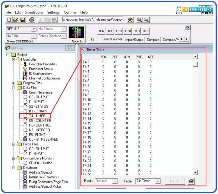
Believing in the essence of timers in ladder logic programming, we come today with a new tutorial in which we are going to show you all about timers, the types of timers, what’s inside timers’ block of parameters, variables, and bits. In addition, techniques for using timers will be explored, and for sure, we are going to practice what we learn using the simulator. So let’s get started with our tutorial.

Timers in ladder logic programming

Guys, this is not the first time we’ve talked about timers. However, this time we are going to look into timers deeply and use the glasses of practical approach. So figure 1 shows the most important types of timers in ladder logic from left to right: the on-delay, off-delay, and retentive timers. There are differences in functionality. However, they all have the same parameters, variables, and bits. For example, the on-delay timer (TON) works by starting counting by getting the high logic state of its input. And bit goes ON when and only when the counter reaches the preset value. While the off-delay timer (OFF-DELAY) employs starting with the high logic of its Done bit once it has a high logic of its input. And when its high input stat is gone and turns to low. It starts counting until reaching the preset value, and then the done bit goes off. On the other hand, the retentive timer keeps accumulating the time while the input is energized until it reaches the preset value, at then the Done bit goes on. You can see, my friends, how are different in functionality to help you get a way for every problem related to timers. Despite that variety in behavior, they have the same data, as you can see in each timer block. So now, what are these data, and how can we utilize them in ladder logic programming? that is what we are going to learn together in this tutorial.

Timer data in PLC

Well! Timer data can be demonstrated in figure 2. You can see guys in the tree view windows below; the data section shows the timers data in which there are dozens of timers you can use through long your program. But what does the data include? Well! The data has timer bits and variables, as shown on the right side of the window. The most important variables are the preset variable (PRE), in which we set the value of the time at which we require the timer to act ON. The other variable is the accumulator variable ACC that we use to know what the counted time is so far. The logic says the timer keeps increments accumulator until reaching the preset value. Okay, then what happens when the accumulator reaches the preset value? Exactly, the timer needs to indicate that he reaches the target.  There are so-called timer bits like the timing bit TT that reports the timer is timing, and the DONE bit that tells the accumulator has reached the preset value. And also the EN bit that shows the completion of execution of the timing instruction.

Most Common PLC Timer Types

Well, timers can be categorized based on their functionality and the way they work. For instance, the ON-DELAY timer starts timing when it gets a trigger signal which is the high state of its input. By reaching the preset value, the output will have been energized as long as the input is high. Please, guys, see the timing diagram in Figure 3 which depicts the timing diagram of the input and output of the ON-DELAY timer. It shows the timer contact goes on after counting the preset time value since it receives a high logic on its input coil.

The second but same important kind of timer is the OFF-DELAY timer. This timer starts energizing its contact or output from the moment it receives high logic input. Then after that input goes low, the output remains high in the logic state for as long as the preset value has been specified. Please, my friends, find the operation cleared in figure 4 below, which demonstrates the operation by the language of the time. In this example, the timer coil has been energized, and its contact goes high. And when the coil de-energized, the contact remained high for 5 seconds which is the preset amount of time of the timer.

The third timer we are going to show today is the retentive timer. So what does that timer do? Well, that timer accumulates the time whenever its coil is ON. The timing diagram is shown below in figure 5.  More details about the timing diagram of retentive timers, what figure 5 demonstrates. You can notice, my friends, as long as the input is high, the timer accumulator keeps accumulating the time until one reset signal appears, then it resets the time. But it returns back, accumulating the time whenever the input is true.

Now we will show some examples to let you understand how to employ the timer variables and bits as well. Figure 6 shows the timer block of an OFF-DELAY timer. You can see, guys, the timer’s name is T4:1, the time base is set to 00.1, and the preset value is set to 100, meaning it is designed to time for 10 seconds that can be determined by multiplying the time base to the preset value. Also, you can see that the first rung used input I:1/0 to enable the timer by energizing its coil. Rungs 1 to 3 show how you guys might use the timer bits. For example, in rung number 1, the enable bit of the timer is used to energize output O:2/0. Similarly, the timing bit TT of the timer is utilized to turn on output O:2/1 in rung 002. While the done bit DN energizes output O:2/2 as in rung 003.

Simulating one example

Here it is the simulation of one example to show how the timers bits and variables can set and used. In figure 7, the timer of type on-delay T4:4 is used and set to time for 10 seconds by setting the preset to 100 and the time base to one-tenth 0.1. the timer’s bits are used as you can see my friends to activate different outputs.

Example showing timers types

Another example demonstrated in figure 8 to show the on-delay and off-delay timers working together to fulfill the requested logic.

Retentive Timer example in Ladder Logic

Figure 10 shows an example to demonstrate the utilization of a retentive timer type. You can see the timer block of the retentive timer RTO and how it is accumulating the time whenever the input is high without resetting when the input is turned off.

Timers programming techniques

Going to one of the most important parts of our tutorial is how professionally you guys can use the timers to solve whatever problem you have. The techniques to use timers that come with experience. For example, figure 11 shows the cascading timing technique in which you can use multiple timers based on each other in a cascading way. You see, guys, how timer T4:2 depends on the Done bit of timer T4:1 in cascading approach. Why do we need to use two timers in such a way when we can use only one with a preset value equal to the sum of the two timers? That’s smart to be asked. But the answer also is intelligent, which tells us we might need to do some action in between. For example, when timer number one has done timing, we might energize one output, and after the second, we perform another action depending on the first timer.

Reset the timers in Ladder Logic

Figure 12 shows the technique to reset the timer by having one normal close contact in the way of its input to control energizing the timer coil. In that very example demonstrated by figure 12, the timer Done bit itself is used to reset the timer, meaning that when the time contact acted ON, it is the time to reset the timer and like that, we can guarantee the timer keeps repeating the process forever.

And at that point, I would like to thank all my friends for following me till the end of that tutorial, and I hope you have learnt some knowledge and enjoyed practicing one of the most important topics in ladder logic programming, Timers. For recapping have nailed the timers by demonstrating the variables and bits of the timers and the types and techniques of using the timers to flexibly and professionally can deal with different situations and solve any problems related to using the time.

Engineering Your Way to a Successful Project: Writing Tips and Tricks

Engineering projects are a crucial part of a student's engineering degree. Writing a project report is an essential part of any engineering project. The final step provides a summary of the project and its results. A good project report can help students get better grades and advance their career prospects. In this article, we will discuss the importance of engineering project writing and the steps involved in writing a successful project report.

What is Engineering Project Writing? 

Engineering project writing is a form of academic writing used to document an engineering project's progress. This type of report usually includes findings, conclusions, and recommendations. It should provide a clear and concise overview of the project and its impact on society. The report should be written in an organized and professional manner.

Why is Engineering Project Writing Important? 

Engineering project writing is important because it plays an essential role in the success of an engineering project. It provides detailed documentation of the project, its findings, and its results. This helps project managers and stakeholders to evaluate the success of the project. It also helps to demonstrate to potential employers and clients the skills and knowledge of the engineering team. 

https://codete.com/ provides comprehensive IT services and solutions that help companies innovate and increase their competitive advantage.

Steps in Writing an Engineering Project Report 

Writing an engineering project report can seem like a daunting task. However, following a few simple steps can make it easier and more effective. 

1. Gather the Necessary Information: Before you start writing your project report, it is important to gather all the necessary information. This includes details about the project, its goals, the team, its progress, and the final results. 

2. Outline the Report: Once you have all the necessary information, it is time to create an outline for the report. This will help you organize your thoughts and ensure that your report is structured and coherent. 

3. Write the Introduction: The introduction should provide a brief overview of the project and its purpose. It should include an explanation of the project's objectives, the team's involvement, and the results achieved. 

4. Write the Body: The body of the report should provide a detailed description of the project and its results. It should include information about the team, the methods used, the results achieved, and the conclusions. 

5. Write the Conclusion: The conclusion should provide a summary of the project and its results. It should also include recommendations for future action. 

6. Proofread and Edit: Once you have written the report, it is important to proofread and edit it. This will help ensure that the report is error-free and that it communicates the project's results effectively. 

Conclusion

Writing an engineering project report is essential to any engineering project. The final step provides a summary of the project and its results. A good project report can help students get better grades and advance their career prospects. By following the steps outlined above, you can create a successful engineering project report that will help you demonstrate your skills and knowledge. Encouraging students to use their engineering project writings to showcase their technical prowess is also a good idea. It will also help in the post-graduation job search. 

In the end, it is important to remember that engineering project reports should be clear, concise, and organized. With the right approach, you can create a report that will help you stand out from the crowd and advance your career prospects.

How to use Data Types in MATLAB?

Hey geeks, welcome to the next tutorial about MATLAB software and language. In this series, we have been working on MATLAB with the basic information and in the previous lecture, we worked deeply with the workspace window and learned about the functions and variables that are commonly used when we are dealing with the data in the command prompt. In the present lecture, we are dealing with the data types in MATLAB. This is related to the command prompt window but the reason why I have arranged this lecture after the workspace practice is, there will be different steps where the usage of the workspace will be included. Other details will be cleared when you will take this lecture yet, have a look at the list of content that will be included in this tutorial:

  • Introduction to the data types.

  • What are some important data types that we will use in MATLAB coding?

  • What is meant by the numeric and text data types?

  • How can we make tables in MATLAB?

  • Why data types are important in programming?

  • How can you say that different programming languages have different data types?

What are Data Types

In almost every programming language, the data types are the important topics and these do not end with a single lecture, but knowingly or unknowingly, you have been using these data types in the practice of your MATLAB codes. So, first of all, I am going to provide you with the proper definition of data types:

In programming, a data type is a classification that specifies what type of value a variable has and what mathematical, relational, or logical operations can be performed on it without causing an error.

If this definition seems difficult to you then do not worry, all the details will be clear to you when you will see the example of each of its types. When you use any type of data in your programming language, it is not of the same type but varies according to your needs and requirements. There are several data types but we will discuss the basic and most important in this lecture so we may elaborate on each and every type effectively. But before going into the examples, I am dividing the whole languages into two main classes:

  1. Strongly typed programming languages

  2. Weakly typed programming languages

Both of them have different ways of implementation, so have a look at them.

Strongly Typed Programming Language

Strongly types data types are the ones in which there is a restriction of using the particular variable is used according to its data type. You must know, MATLAB is a strongly typed programming language because you can not connect irrelevant data types together in it but you have to use the same data type all the time when connecting two or more together. 

Let us have an example. We have seen the concatenation process in the previous lecture where two digits may have the arithmetic operation if they belong to the same class that is the same data type. So, if you try to connect an integer with the string, it will throw an error. 

Weakly Typed Programming Languages

The weakly typed data type, contrary to the first case, can be used in an easy way because there is the independence to use the different data types together with the help of any operation. It happens in only a few programming languages and it is not relevant to our MATLAB so I am not explaining it more. 

List of Data Types in MATLAB 

Finally, I am going to describe the detail of almost all the data types that you are going to use in the MATLAB throughout your course and with the help of this knowledge, you will be able to use these data types according to your needs and at the final result, you will code in the best way. So, have a look at the detail of each data type. 

Numeric Types

The first and most basic type that we all know is the numeric type. Here, if you are new to programming, I must mention that numerics also has different classes in it and two of them are:

  1. Integer

  2. Floating Points

  3. Single

  4. Double

Integers: 

The numbers that mostly we use in our daily life are integers we have read the definition of integer in our begging classes that these are whole numbers ranging from positive infinity to negative infinity but we are mentioning here the definition because I want to make sure you use the code without any confusion.

Floating Points:

The floating points are the numeric types that contain the part, less than one in them, in addition to the whole number. This portion is then added in the form of points. To memorise well, you can think that every integer has zero additional points than a whole number and the floating point digits additional to that whole number. 

Single:

It is the array of single precision numbers that occupies less memory because it just stores the first digit after the point. Basically, it is the subclass of the floating number and is less accurate than the other case that we are discussing next. It is less likely to choose and if the user is not using scientific information, then they use the single integer to fix less memory for their data type. For instance, the result of the calculation will only be shown just after one point such as 12.3 only.

Double:

It is also the class of the floating point that stores more memory than the single data type. It is more accurate because it can store the two numbers after the floating point. For example, if you choose the double floating point, it will provide you with the results as 12.34. The numbers having a value more then this will require to be saved int eh data type of character or string according to the length of the number.

IntX numbers:

These are the interesting types of data in which users may get the integer type of his/her own choice. There are different int X numbers where the X varies from 8 to 64. So, by applying the numbers 8, 16, and 64 with the X separately, you can fix the memory space of your own choice where you can easily declare the variables. 

For example, if you want to declare the variable of the size 8 bits, you will write the following command: 

int8(value)

It will create a space of 127 numbers. The total size of this 8 bits data is one byte and it occupies the space to accommodate 0 to 127 numbers. By default, if you do not specify, it is the unsigned data that starts from 0 to 127. 

If you want the numbers with the same memory size but the ones that include the negative sign as well, you can do so by changing the command to:

uint8(value)

Now, I am writing both these commands in the command prompt and with the help of the workspace window, you can compare the values stored in both these cases.

Similarly, you can check for the int16 and int64 as well and the workspace window will tell you about the detail of each and every case with the signed and unsigned value. 

If you do not want to use the workspace window, you can find the details of your data type with the help of whos command that we have learned in the past lecture.

So in this way, it becomes easy to search and get the results of details of any kind you want about the particular data type. 

Class of The Data Type

It is time to tell you about a useful and simple command to get the class of the data type easily if you do not remember the size or data type of your variable. So, the syntax to do so is:

class(variable)

Where the variable amy be any data type, this keyword will help us to find its class.

Keep in mind, the A varialbe was declared by you before using this class keyword otherwise, you will ge tthe error.

Text Data Type

When using the text in the code in any way, you have to use the alphabet, as expected. But, you must know that there are also two types of text data types that are, the same as the numeric type, have a slight difference between them and we use them according to the need of time. Here are these two:

  1. Character  type data

  2. Sring type data

CharacterText:

The character type data is used when we want to declare the variable of the text with relatively less memory space. In simple words, when we want to declare a single alphabet or small sentences, we use the character. The declaration for the characters is as follows:

A=’Tom’

Where the single quotation tells the compiler that we want the space for the character text.

String Text: 

The string text, as you can expect, has more memory space than the character. These concepts are discussed in the last lecture so I am not going to give you unnecessary details and examples.

Tables

Row and column variables are present in the table. Each variable can have different data types and sizes, but they must all have the same number of rows. A variety of functions are used to access data in order to create, edit, and read table data.

Syntax

A=table(column1,column2,....,column(n))

Here, you can easily declare the column's name and after that, you can enter the data according to your choice.

Structure Data Type

Data containers are used in the structure to group related data and their types, which are referred to as fields. Fields can hold any type of data. The dot notation is used to access data in structures.

Why We Use Data Types in Programming?

We know you have an idea that data types are important in programming languages yet, I always use the explanation of the importance of the topic that is being discussed. 

  • The data types are used to occupy a specific amount of the data according to the need of the user. For example, there is no need to reserve the memory space equal to the string data when you need only the data of a single integer. In this way, the program runs slowly and this problem is unbearable if you have a large data in the program or have a slow system than required. 

  • The data types make the code more organized and clean. 

  • With the help of data types, the path of the program is more clear that how the flow is being used from start to end when you are programming your code. 

  • The readability of the program is enhanced with the help of clearly defined data types. 

Data Types in Different Programming Languages

It is an interesting question that must be cleared when dealing with programming languages. We know you have a basic knowledge of programming languages and therefore, I am not explaining from the scratch. But, you must know that it is not necessary that all the programming languages are based upon the same data types. Usually, the code of the programming language is distinguished by its data types and the keywords that we use with the specific syntax.

Hence, it was a detailed lecture on the data structure where we learned a lot about the data types and we have learned a lot of infprmation in differnet ways. All the work was practiacally performed but if you find that something that needs implementation, you should practice it by yourself as your homework. We had a lot of discussion related to the different case where we use some special keywords to find the type or the relation of different data types. Hence, you can now designed you codes according to the required data type. Stay with us for more interesting tutorials. 

Command Window in MATLAB

Hello, peeps! Welcome to another exciting tutorial on MATLAB in which we are discussing one of the most important windows of MATLAB that you are going to use the most. In the previous tutorial, we learned a lot about the basics of MATLAB and the different types of windows that are used in MATLAB and are present on the face of MATLAB when you launch it. There was a piece of interesting information about the basics of this fantastic development environment. This is the next step in the related tutorial in which we study the applications and workings of command windows in depth. Here is a glance at the topics that you are learning about today. 

  • How can you define the command window of MATLAB in detail?

  • What are some examples of commands related to online help?

  • How can you use the useful commands on MATLAB related to the variable?

  • Give the information about the commands related to the files, directories, and the PC that you are using. 

  • What are some examples of the type of equations that are solved in the command prompt?

Thus, let’s start learning.

Introduction to Command Window in MATLAB 

Recall that the command window is the basic window that is shown in the centre of the screen when you fire up your MATLAB, and here, the pre-defined commands are run in the easiest way by merely providing the command and values. If it seems to be normal right now, then maybe you have unclear programming skills because programmers know that in most languages, the commands and functions have to be defined first. 

Not only this, but the command window also performs another responsibility. In some programs, when we are using the edit window, the command window shows us the results and outputs of the calculations, if applicable. The usage of edit windows is not yet discussed in his tutorial, but you can understand that the command window shows us the numerical output and the command’s results when we allow it to do so. 

Using Command Window for Online Help

As we have said earlier, the command window is used for different purposes, and therefore, at the beginning, we are telling you about the different ways to seek official help from MATLAB if you are stuck in any situation and do not know how to tackle it. The good thing about MATLAB is that it provides you with the maximum information and helps in different ways and it is made for students. Therefore, it not only provides you with the terms of help but also defines them in the easiest way so the students may know where they have issues in the calculations. So let’s start the process of finding help in different ways in MATLAB. Just follow the steps given below:

  • Launch your MATLAB software. 

  • Go to the command prompt where the function catalogue is blinking. 

  • Start writing the following commands to check what they do.

  1. help

By writing this in your command window, you will get the list of the commands for which, MATLAB can help you by defining the introduction and codes of that particular command.

  1. helpdesk

It creates a helpdesk for you and directs you towards the MATLAB official page where you can report and find help regarding your issues. 

  1. help topic

This command provides you with help regarding a particular topic. Assume that you want to get help related to MATLAB's "help" command, which was also mentioned above. You can type "help" instead of "topic" in this command. You will get the details all the time. 

  1. helpwin

It is a special command that is used to get the help link and details in a separate window.

  1. lookfor string

This is an interesting command that is designed to provide you with help related to the strings that we will use in the codes. If you are new to this concept, skip it for now because you are going to learn about it in detail in the coming sessions.

  1. demo

It is one of the most amazing commands in MATLAB where you can find demo examples of different types of code by merely writing a single word, and you will be directed to the official page of MATLAB where all the demos of various programs are present. 

  1. whatsnew

If you want to get the Readme files of MATLAB, you just have to write this command in the command prompt and you will get the required output.

  1. why

This command has some different types of work. Every time you write “Why” in your command prompt, you will get a different type of sentence with a different meaning.

  1. home

This is a command resembling the “clc” command where you can go to the start of the command prompt and all the results and writings will be cleared from the screen and you will start writing from the beginning.

  1. global

This command is used to declare the variable globally. In other words, you will not have to declare the variable again and again in different sections, but it will be defined once and can be used anywhere in the program.

Commands Related to variables in and Workspace Information

Here is another category that deals with variable or workspace information, and you can easily perform them as you have practised the commands discussed above. So here is the list of this particular type. 

  1. who

This command is used to get all the variables that are declared in the workspace in which you are working.

  1. whos

If you want to know the variables declared in the workspace along with their sizes, then you will use this command. In this way, by adding only one character, you can also examine the size of the variable.

  1. clc

Sometimes, or I should say, many times, we want to clear the screen so we may try other codes and commands. For this, you do not have to select all the content and then press backspace, but you just have to write a simple “clc” command and all the data will vanish from your screen. But be careful while using this command because once the data is removed, you will never get the same data back.

  1. clear x,y,z

Consider the case when you just want to remove the specific lines of code or the variables and other code that are useful to you. Then you will use the clear command in a specific manner in which you will specify the variables that you want to remove from the screen and the memory. In this way, the declaration and erasure of data become easy.

  1. mlock fun

As we said earlier, it may be a disaster in your code if you clear the instructions in the code that were supposed to be there in the command prompt, and in such cases, you can lock the function by putting the name of that particular function just at the place of “fun” in this command.

  1. clf

As we have defined the figure window in our previous lecture, if you have the results of your code in the form of a figure window and want to close it with the help of a simple command, then simply write this command and the window will be closed.

Commands Related to Files and Directory Information

While using MATLAB, I face some cases where I have to think a lot about the directory and want to get information about different files saved in MATLAB by e. So, I found some interesting commands that tell me the exact information about the directories and files I am using efficiently and in great detail. Some of them are given below:

  1. cd

It changes the current working directory. It seems the same command we use in the command prompt of windows.

  1. dir

The purpose of this command is to see the content of the current directory. 

  1. copyfile

This command is used to copy the content of the files that we are working on. 

  1. rmdir

To remove the current directory from your MATLAB, we use this simple command. 

  1. what

It is an interesting command. You can access all the data on which you are working with the help of this simple one-word command.

General Information with The Help of Command

Yes, it is right. You can find general information about your computer with the help of commands in the command prompt. MATLAB does not only work as simple software that works separately from the other functions of the computer but it is also connected to the internal system of your PC. For instance, if you want to know the basic information about your PC, then you have to see the commands given below:

  1. clock

This is my favourite command. You can have the time and date in the form of a vector wall clock by writing this on your command prompt.

  1. ver

The licence and version of MATLAB can be seen with the help of this command.

  1. bench

This command must be used when you want to compare your computer to other devices while MATLAB is running. 

  1. computer

Many times, people do not know the type and specifications of the computer, and they can find them with the help of this command.

Keep in mind, just like some other programming languages, MATLAB is a case-sensitive language, and therefore, if you put these commands with different spellings or change the way of the writing that they were supposed to be, you will get an error. Usually, if the case or one or two characters are changed, MATLAB gives you the suggestions and, therefore, you can easily press the enter key and get the required work from MATLAB. Otherwise, you have to write the exact command.

Examples of Numerical Problems in MATLAB Command Prompt

Now, you know the basics and easy commands that are used in the command prompt, you can easily use the command prompt for different numerical problems. Now, we are starting MATLAB and solving the simplest numerical problems, and then we will move towards more complex problems. 

First of all, have a look at the equation that we are going to solve in MATLAB.

4x + 2 = 18

Here, x is the variable, and we want to find the value of this variable. So, we are using the following code to get the required output. You must know that the 18 on the right-hand side is moved to the left-hand side and, therefore, the equation becomes

4x + 2 - 18= 0

4x -18 = 0

We will write this problem in MATLAB and will get the results:

As you can understand with the help of this image, we are declaring a variable with the name “equation” and then feeding the values of x and the constant into it. By default, MATLAB reads the equation from the right side, and it reads the rightmost value as constant, and after that, moving towards the left increases the value of the polynomial. So, MATLAB understood that 4 is the value of variable x. 

Consider another equation that is shown as:

34x4 +45 -12=0

Here, you can see that the cubic value of the variable x is missing, so in place of this value, we will write zero. So the code and the output of the equation given above are:

You can use any word instead of "equation" to declare the equation. Yet, be careful, you have to write the exact word in the root command to get the desired results. The roots command simply takes the equation, solves it, and provides us with the result instantly.

So, it was the day when we learned a lot about the command prompt and saw some amazing commands related to MATLAB that, when written on the command prompt, give us the useful required information, and we checked most of them during the lecture. Your homework is to check the missing commands and get the results related to MATLAB. We will do some complex calculations in the next session, and now you are ready to get the answers to the complex calculations and codes, so stay with us for more action.

How to install PCBWay Plugin for KiCAD PCB Software?

Hi Friends! Hope you’re well today. Happy to see you around. In this post, I’ll walk you through How to Install PCBWay Plugin for KiCAD PCB Software.

Before we move further, let’s get a brief overview of KiCAD PCB Software. 

KiCAD is a free and open-source electronic design application mainly developed to draw schematics and PCB layouts. It is open-source which means anyone can use it to develop and modify electronic designs. The tool can effortlessly run on Windows, macOS and Linux. The main window of the application comes with 8 different software tools used to make PCB layouts and schematics. 

Hope you’ve got a sneak peek at the software. Now we’ll get to know how to install the PCBWay Plugin for KiCAD.

How to install PCBWay Plugin for KiCAD PCB Software?

When you install PCBWay Plugin for the KiCAD, you can instantly send the PCB layout to the PCBWay for the production of your required boards.

To install PCBWay Plugin, go to the KiCAD website. The following page will appear when you visit the website.

Click the “Download” button encircled in red. When you click it, the following image will turn up.

Here you will see the list of operating systems you can pick from. Click the required system. For instance, if you click the windows operating system, the following image will come up.

Based on your system requirement, you can choose between the 64-bit and 32-bit. When you click anyone of them, the following image will come up.

Here you’ll see the different downloading links based on your location. The recommended option is the “Worldwide” with the link from GitHub.

When you click this option, the software will start downloading. 

Once downloaded, right-click the software and click “open”. 

When you click it, the window will open up. Then click the “next” and then “install” when you click it, your installation will start as follows. 

Once installation is completed, click the “Finish” as follows.

Then start the software. Once you start it, the following options will appear. You can either import the settings from the previous version or you can start with default settings to start it from scratch as follows. 

When you start with the default settings, the following window will appear. Go to the “Tools” section and select “Plugin and Content Manager”.

The list of plugins will open up. Scroll it down and find the “PCBWay Plug-in for KiCAD” as follows.

Click “install” and then click “Apply Changes” and the PCBWay plug-in for KiCAD will be installed through which you can send your PCB layout to the PCBWay with just one click.

When you click PCBWay Plug-in button on Kicad, the following files will be exported to your project:

1. Gerber files used for production

2. IPC-Netlist file

3. Bom-file that comes with the information of components

4. Pick and Place-file in assembly

When you click "Save to Cart" to immediately placing an order after you upload the files, the PCBWay team of professionals will cross check the files before starting the final production.

About the Company PCBWay

Choosing the right manufacturer is tricky, especially when everyone claims to be the best in the market. In this read, we’re covering the most renowned PCB manufacturing company that has been serving the electronic industry for over a decade now.

PCBWay is a china-based PCB fabrication house. It is a one stop shop for both PCB and PCBA (printed circuit board assembly). From single layer, double layer and multiple layers to flex, rigid and rigid-flex boards, they have you covered. They come with 50 engineers on board that make sure the manufactured board run through a stringent inspection processes. They ensure the customers’ demands are properly met so they keep coming back for what the company has to offer.

Deliver what they Promise 

They strive to meet the customers’ expectations by standing on their words. A few customers have seen the slight change in price of the final product. But that’s not their fault. It’s on the customer side since they didn’t pay special heed to matching the parameters of the production files. So, keep in mind… before you submit an order, make sure the parameters of Gerber and production files exactly match with the ones you put online during the submission of order in an instant quote. If they don’t match, you may see the slight change in price for the production of the final product. 

Keep you Updated

When your order process is complete, they will send you three emails: First email will tell you about the order status, whether it’s been approved or rejected. Second email is about the successful payment and production management and the third one is for the products being shipped. This way, you remain thoroughly updated about the processes your product will go through. Know that, you can ask for the change in parameters of the product before the production process is scheduled. However, if your product already goes through the initial stages and has reached the certain stage of product, you cannot ask for the change and the parameters will remain the same you initially put during the order submission. 

High Delivery Rate

They value your time and money. They know how it’s important to deliver products on time so folks working on their electronic projects can develop and execute their projects in a timely manner. PCBWay takes pride in achieving a 99% delivery rate. They work 24/7 from Monday to Friday to make sure the final products are delivered as promised.

V5 Members and Reward Points

The best thing about PCBWay is that when you become their regular customer and buy more PCBs, you become a part of their V5 members. These members can enjoy 5% off on upcoming orders. Additionally, you get Beans when we put your order online. Beans are rewards points that come in handy to buy electronics products from their online shop.

That’s all for today. Hope you find this article helpful. If you have any questions regarding the installation of the PCBWay Plugin, you can ask in the section below. We’d love to help you in the best way possible. Thank you for reading the article. 

Applications of Matrices in MATLAB

Matrices are an essential topic in different fields of study, especially in mathematics, where you have a bulk of data and want to organize, relate, transfer, and perform different operations on data in a better manner. We have studied a lot of types and operations on the matrices and have worked on different types with the help of MATLAB. Today, we are here to present the applications of the matrices in different fields of study to clarify the importance of this topic. So, have a look at the list of topics we are going to learn. Yet, first of all, I am going to describe what a matrix is.

What is a Matrix?

In the fields of physics and mathematics, there is the use of different types of numbers in groups of various types. In order to organize the data into a manageable format, matrices are used. A matrix is a rectangular array of numbers that are enclosed by a square matrix (or, in some cases, parentheses). 

The information about the numbers of rows and columns is called the order of matrices, and on the basis of this information, we can recognize different types of matrices. The types, in turn, are used in different applications because of their unique behavior. By changing the order of the matrix, the properties and working of the matrices changes according to the changes. Mostly, square matrices are used in different applications.

It is interesting to know that in the early days of matrices, these were considered arrays. With the passage of time, when they were involved more and more in different research and methodologies, matrices gained popularity. Because of the ease of usage, this popularity is not going to end. So, have a look at the different types of fields where matrices are used in different ways but before going into details, you must know, these fields are not only dependent on the matrices but the normal functioning of these fields include the usage of matrices in different ways. 

Applications of Matrices

As we have said earlier, matrices are used to deal with massive amounts of data better. The matrices that we have learned and seen till now are of very minimum order, and these are kept simple for the better concepts in easy ways, but in practice, we have seen that there are gigantic matrices with complex data in them, and at that point, it is difficult to solve and save them manually. Have a look at the different fields of practical life where matrices are used in a routine.

Matrices in Cryptography 

Data cryptography is an important department in data communication in which the encryption of the data is an important process. It is done by using different keys and codes to secure the message and communication in a better way. A large amount of data is sent and received by different parties, and the encryption techniques also require some other space as well. Matrixes are used to make sure that all the data and its codes are stored in a better way. These matrices 

save the keys of the encrypted data to decrypt them on the receiving end and in this way, matrices play a key role in cryptography.

Use of Matrices in Wireless Communication

We all know that in wireless communication, usually air is used as the medium to send and receive messages from one point to the other. In this process, matrices are used to detect, extract, and process the information about the message that is to be delivered. Here are some other uses of matrices in this department:

Signal estimation and the detection of the problem during communication are done with the help of matrices. 

  • Sensor array signal processing involves the matrices.

  • In the processing and representation of a digital image, matrices have a great role. 

  • Radar signals

  • Underwater surveillance

With the help of matrices, wireless communication is done efficiently, and understanding the code becomes easy. Think about the case if the data of different queries are not used in the form of a matrix, then finding the data of a simple command would never be organized. 

Matrices in Mathematics

The use of matrices in the field of mathematics is not new to us. We all know that it is a basic concept in mathematics and a great variety of concepts of matrices are used in different ways while solving mathematical problems. One of the major use in mathematics is a solution of linear equations with the help of matrices. The complex and time taking equations can be easily solved with the help of rules of matrices in different ways. 

In engineering and other related fields of mathematics, matrices are the basic concepts and it is used in different ways to make the working of the system better manner. We have seen different cases in which the matrix is used as the alternative method to find the unknown value because it is a more organized way and the great number of research resulted in different theorems and laws therefore, the long calculations are minimized to their result by simply using the theorems.

Matrices in Computer Graphics

One of the amazing applications of matrices is in the form of computer graphics where the pictures and the graphics comprise pixels and the array of these pixels and points are arranged in the form of matrices for easy transformation and working. Overall, you can say that in computer graphics, each digital image is treated as a matrix. Therefore, different types of operations used in the matrices are applied to the graphics with great ease. Not only in the dimensions and the sizes but also for the colors of the images, matrices are used to store and reuse the values for the images and graphics. For example, in the CNN technique, different types of matrices are used. For the greyscale image, only a 2D image is used and if one wants to get the RBG system image, there is a need for a 3D matrix. 

Three Dimensional Games and Matrices

Gaming is one of the most important filed in graphics and when we talk about three-dimensional games, matrices are important there in order to alter the 3D space in different ways. For this purpose, if we use simple words, the conversions between the 2D and 3D matrices are used by different techniques, and therefore, we get the final output. Moreover, the quality of the result depends upon the way you use the data in different ways. 

Matrices and Geology

During the seismic survey in geology, matrices are used in a great way. For real-time surveys of different areas of common real problems such as mortality rate, population, the number of people in different areas of the world, and other specific counting related to real-life problems involve the use of matrices because it becomes easy to deal with great data using different operations on the data.

The Matrices in the Field of IT

In different Information technology organizations, matrices are used to execute and search the different queries. The IT security system needs to have a secure way to deal with all the information and once saved, data is to be retrieved in an efficient way with the help of minimum commands. If the data is not present in the form of tables, or we should say, in the form of matrices, organizing, storing, retrieving, and dealing with the data will be like a nightmare. 

Using Matrices to Find the Collinear Points

It is one of the procedures in mathematics in which the values of collinear points are found with the help of matrices. If it seems simple at this time then you should think of the case where gigantic collinear points are found with the help of matrics with the help of different software and these points are in return used in different ways. 

Pre-allocation of Matrices in MATLAB

As we have said, matrices make the working of daily life data and complex calculations easy. We read different types of commands about the matrices when we were learning about their functioning and therefore, we can now use them in a simple program to prepare the code in which the matrix is used for the pre-allocation of the data in a simple way by using limited lines of codes. Trus, have a look at the code given below:

Code:

p=zeros(5)

p(1,:)= [ 3 6 2 8 7]

for i=3:4

p(i,:)=p(i-1,:) +1

end

Output:

Understanding the MATLAB Code

In this code, we have used a simple function of zeros and used a loop to execute the whole instruction. Let us discuss both of them in detail:

Zeros Function

It is a pre-defined function of MATLAB that is used to make a null matrix of the required dimensions by using just a simple signal command. For the null matrices, there is the condition that the square matrix should be used.

For loop in Matrix

There are certain loops used in the MATLAB and with the help of this for loop, we just have to simply follow the syntax given below:


for index = value

statement

end

Here, the index value is the starting point where we want to start the matrix formation and the statement is the condition that we want to be executed while the formation of our matrix. If it is not clear right now in your mind, just have a look at the flow of the program.

  • First of all, we have used the zeros function to allocate the space in the memory according to the requirement. We have used the square matrix which has the order of 5 by 5. 

  • I wanted to pre-allocate the values in the matrix row after the row therefore, we simply changed the values of the matrix p formed before from 0 to other values defined by us. If you are not familiar with this function, have a look at the notation given below:

p(a,b)

Where,

a=number of row

b=number of column

As we did not want to alter any value in the columns so we have used a colon in its place. 

  • By using the for loops, we have specified that the index value starts from 3 and ends and 4. 

  • In the next step, we are using these index values and specifying to MATLAB that we want to change the values of the 3rd and 4th rows only and the program ends. 

  • MATLAB does this task step by step and changes the null or zero values of the matrix p into the required pre-allocated values in the matrix.

  • For the best concepts, we have changed the values of just two rows and the other matrix remains the same.

Larger versions of these kinds of procedures are used in diverse ways to recognize, store, and use the data in a better way, and with the help of this short program, we have seen a glimpse of a real-time application in which a matrix can be used to pre-allocate the different values and people can have benefit from it.

Trus, today, we have learned a lot about matrices and their applications. We have read great information about matrices in the past lectures and it was quite interesting to know how can you use these basic pieces of information in a better way and how people are working on the matrices to make their daily tasks easy during their professional life. We have seen different departments where matrices are making the work easy and more efficient. Most of them can not work without using matrices. Moreover, one must have the idea that many times we use matrices in our daily life unintentionally. As we have said earlier, 3D games require the involvement of a matrix. So, when your child is playing the game, he or she is enjoying the application of the matrices without knowing it. In the end, the small program was helpful to understand how little programs and the working of matrices are helpful to perform different tasks automatically.

Special Types of Matrices in MATLAB

Hey students welcome to another tutorial in The Engineering Projects where we are going to learn a lot about matrices. If you are a beginner to the metrics, then you should go to learn the fundamentals of matrices. Yet, if you know the basic introduction, you are at the right lecture because we are learning about the special kinds of matrices and you are also going to see the matrices in action using MATLAB. So, here is a simple list of today’s topics. 

  • What is a matrix?

  • How can we identify the matrix with the help of its general form?

  • What are the different types of matrices?

  • What is the concept of transpose while dealing with matrices?

  • How can we implement these types of matrices in MATLAB by different commands?

What is a Matrix?

A matrix is a type of array that stores data of the same kind. It has great importance in the world of technology and it is defined as:

"A matrix takes the form of an ordered rectangular array surrounded by a square bracket and has entries of the same kind in the form of real or complex data."

To perform different operations on the matrices, you just have to apply them to the whole matrix at once; there is no need to apply them to all the entries one after the other. This will make sense when you see the matrices in action. 

Till now, we have learned about the basic introduction of the following types of matrices:

  • Row matrix

  • Column matric

  • Square matrix

  • Rectangular matrix

These are the basic types irrespective of the elements or entries present in them, and now, we are going to discuss some types that have the features of these matrices but the entries in them are in a specific pattern, so they are considered the special kinds of matrices. Before going into the details of each of them, there must be the foundation of a concept of a general form of the matrix. 

The General Form of the Matrix

To examine the location of a specific element, we use the terms "rows” and “columns” where

  1. Rows are the horizontal entries of the matrix.

  2. Columns are the vertical entries of the matrix.

A specific element is the part of a row and column at a time and to mention the location of an element, it is important to know the information about both of them. So, in the general form, a three-by-three matrix is shown as:

Where

  • A= name of the matrix
  • a= elements of the matrix A

Notice that a has two numbers with them in which the first number denotes the rows and the second one is the number of columns. To make it easier, we denote rows with i and columns with j. So we can say,

  • aij=a23=element of the second row and first column

Keeping this concept in mind, now it is easy to understand the types of matrices in which the value of the elements matters. Have a look at some of these types.

Identity Matrix

The identity matrix is a special kind of matrix having the arrangement of entries in such a way that all the diagonal entries are one and the remaining ones are all zero. In this way, we get the matrix of the form:

You can observe that for an identity matrix, the elements where i=j are all ones, and all the elements other than this are zero. There are certain applications of the identity matrix and you will know them in the upcoming lectures. 

Zero or Null Matrix

Here is an interesting type of matrix. This matrix has all the entries zero and no other value can be found in this element. So we assume the zero or null matrix as:

Where the sequence of the matrix can be any. No matter whether it square, row, or rectangular matrix. 

Singular Matrix

A singular matrix is the type of square matrix that has the determinant equal to zero. It is possible in the condition when all the entries of the matrix have the value one.

We all know the procedure to find the determinant. So, taking the determinant of this matrix C, we provide ourselves with the following calculations:

|C|=1x[(1x1) - (1x1)] - 1x [(1x1)-(1x1)] + 1x[(1x1)-(1x1)]

    =1x(1-1) - 1x(1-1) + 1x(1-1)

    =1x(0) - 1x(0) + 1x(0)

    = 0 - 0 + 0

    =0

So in general, we say, in a singular matrix:

|C| =0

Non-singular Matrix

A non-singular matrix, on the other hand, has entries in such a way that the determinant is never zero. So, we can say, most of the matrices are included in a non-singular type of matrix. Here is an example of a non-singular matrix, which we have also mentioned in other categories.

|C|=3x[(-6x7) - (1x-1)] - 0x [(2x7)-(1x4)] + (-5)x[(2x-1)-(-6x4)]

    =3x(-42+1) - 0x(14-4) - 5x(-2+24)

    =1x(-41) - 0x(-10) + 5x(22)

    = -41 - 0 + 110

    =69

Hence, we can conclude for the non-singular matrix that if A is a non-singular matrix, then:

|A|≠ 0

Diagonal Matrix

The concept of diagonal was used in the identity matrix, but it is a slightly different case. A diagonal matrix is one that has all the entries, other than the diagonal, equal to zero. The values in the diagonal may be anything. 

Here, one concept must be clear. In some cases, all the diagonal values except one may be zero, but it will still be called the diagonal matrix. In other words, by changing even one of the values in the null matrix, we can convert it into the diagonal matrix. 

Scalar Matrix

A scalar matrix has all the diagonal values the same, no matter what the value is, and all other values are zero. So, in the scaler matrix, three conditions must be satisfied:

  1. The values other than the diagonal are all zero. 

  2. The values in the diagonal must be non-zero.

  3. All the values of the diagonal are the same, no matter what the value is. 

  4. The matrix is a square matrix.

If one of the conditions is not satisfied, it is not a scalar matrix. 

Upper Triangular Matrix

This is an interesting type of matrix. The upper triangular matrix can be recognized when all the entries below the diagonals are zero and the entries above the diagonal are non-zero. So we get the matrix as:

The value in the diagonal must be non-zero for at least one value. And the 

The Lower Triangular Matrix

As you can guess, the lower triangular matrix has non-zero values in the lower elements than the diagonal. The values presented in the upper portion of the diagonal are all zero. So the lower triangular matrix looks like this:

Transpose of a Matrix

This is another concept in matrices that is important to discuss here because some types of matrices depend upon it. We know that a matrix has i rows and j columns. Then, the transpose of the matrix is defined as:

The transpose of matrix A, denoted by AT , is obtained when the rows and columns of matrix A are interchanged no matter what the total number of rows and columns. 

This concept is used in different ways, and the results obtained are important. To understand well, you must know, that a rectangular matrix of order 2 by 3 will be converted into a matrix of order 2 by 3 when the transpose is applied to it. 

Symmetrix Matrix

It is a special kind of matrix that involves the procedure of transpose. A skew-symmetric matrix is one that has the arrangement of elements in such a way that applying the transposed result in the matrix that has the same entries and same order. In other words:

AT=A

So, the skew-symmetric matrix is always a square.

The Skew Symmetrix Matrix

Here is another kind of square matrix that involves the transpose, and it is slightly different from the one discussed just before. This type of matrix, after taking the transpose, results in a matrix with all the negative values. So we define this in a simple way as

AT=-A

Harmatian Matrix

A hermitian matrix involves complex numbers in it. That means some, or all the elements of a matrix A are complex numbers, and the transpose of that matrix A results in the transpose of a conjugate matrix. So, the following conditions are applied to the hermitian matrix:

  • It is a square matrix.

  • It involves complex numbers.

  • A conjugate of the matrix is obtained. 

  • The resultant matrix has the conjugate values.

    The Skew Harmatian Matrix

    A skew hermitian matrix, with the complex conjugate, is the one that involves the negative values of the original matrix ( the one before the transpose procedure). It will be crystal clear to you when you examine the case given below:

    Special Matrices in MATLAB

    Are you enjoying the different types of matrices? Matrices are fun in MATLAB, it is good practice if we attempt all these types in MATLAB. Notice that, these types follow a specific sequence. Hence, MATLAB has a special function designed for the user with the help of which, one can have all these types by simply writing some commands. But it would be helpful if you understood the commands first.


    Command

    Description

    eye(a,b)

    It creates an identity matrix.

    Where

    a=number of rows

    b=numbers of columns


    triu(A)

    It converts the matrix A into the upper triangle.

    tril(A)

    It converts matrix A into the lower triangle.

    null(a,b)

    It creates a null matrix. 

    Where,

    a=number of rows

    b=numbers of columns

    ones(a,b)

    Creates the singular matrix having the rows a and columns b. 

    diag(A)

    Used to get only diagonals of the matrix provided by you as A.

    sort(A)

    Sort the elements of the matrix A in the ascending order column-wise.

    A’

    It takes the hermitian of a complex matrix A.


    Follow the procedure given below to perform the tasks.

    • Start your MATLAB software. 

    • Go to the command window.

    • Start typing the codes given below and get your desired matrix.

    A=[ 2 7 4; 5 11 5; 3 8 23]

    • Notice that we have a square matrix now. It will help us in different operations. So let’s start using different operations. 

    • Write your first command.

    IdentityMatrix=eye(3,3)

    • It will create an identity matrix with the name IdentityMatrix with three rows and columns.

    • Similarly, write the command given below:

     UpperTriangularMatrix=triu(A)

    • It's time to create the lower triangular matrix. So write the command.

     LowerTriangularMatrix=tril(A)

    • For the null matrix, we are going to use:

    NullMatrix=null(2,5)

    • For the singular matrix, we are using the following command:

    SingularMatrix=ones(3,4)

    • If you wish to have a diagonal matrix of A, write the command:

    DiagonalOfMatrix=diag(A)

    • To sort your matrix A, we are using the command given below:

    SortMatrix=sort(A)

    • If you want to find the hermitian of the matrix, first you have to introduce the complex matrix in MATLAB. So we are writing the following matrix:

    B = [1+j; 1-j; 2-j; 1+2j]    

    • Now, by simply applying the command, we can get the hermitian of this matrix.

    HermitianMatrix=B’

    Thus, today’s lecture was full of different types of matrices, and many of them were new to us. We began with the definition of the matrix, then we saw different types of it where the data or the elements of the matrix were important. Many of them have conditions where the order and location of the elements are important. The concept of transport in the matrix was new to us, and by using it, we explored different types. In the end, with the help of different commands in MATLAB and with the help of practice, we sharpened our concepts. There are different and interesting types of matrices, and we are going to explore all of them in our upcoming lectures.

    Syed Zain Nasir

    I am Syed Zain Nasir, the founder of <a href=https://www.TheEngineeringProjects.com/>The Engineering Projects</a> (TEP). I am a programmer since 2009 before that I just search things, make small projects and now I am sharing my knowledge through this platform.I also work as a freelancer and did many projects related to programming and electrical circuitry. <a href=https://plus.google.com/+SyedZainNasir/>My Google Profile+</a>

    Share
    Published by
    Syed Zain Nasir