Hello friends! This tutorial continues our financial calculations in MATLAB project. We will move from expected returns and covariance to portfolio allocation, performance measurement and a complete Black–Litterman update.
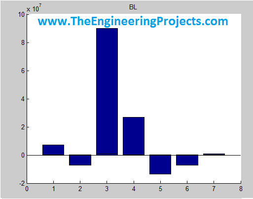
The central idea is to begin with a reference portfolio and the returns implied by it, then combine those returns with explicitly stated views. We must also describe how uncertain the views are. A bar chart of implied returns alone does not complete the Black–Litterman calculation.
We will retain the original project's teaching sequence and historical figures while correcting its treatment of backtesting and portfolio risk. The numerical example below uses hypothetical assets and assumptions for learning. Information about the earlier implementation remains on the original project page, without assuming its historical price or software dependencies remain current.
Review the Inputs From the Previous Tutorial
Start with a matrix of aligned simple returns. Rows represent observation periods and columns represent assets. Prices, exchange rates and returns must share a consistent valuation convention. If the investor's reference currency is US dollars, the return series should reflect the chosen dollar exposure, including currency movements where applicable.
Use a fixed asset order throughout the calculation. The columns of the return matrix, entries of the weight vector, rows and columns of covariance, and columns of the view matrix must all refer to the same order. A dimensionally valid multiplication can still be economically wrong if those labels are mixed.
| Symbol | Meaning | Dimensions for n assets and k views |
|---|---|---|
| Sigma | Asset-return covariance | n by n |
| wRef | Reference portfolio weights | n by 1 |
| pi | Implied expected excess returns | n by 1 |
| P | Assets involved in each view | k by n |
| q | Expected value stated by each view | k by 1 |
| Omega | Uncertainty covariance of the views | k by k |
In the worked example, all expected returns and covariance inputs use an annual modelling convention. Returns are decimal fractions: 0.06 means 6%. Multiplying returns by 100 changes covariance by a factor of 10,000, so mixing decimal and percentage units can overwhelm every other modelling choice.
Step 6: Define the Allocation Objective
Before optimizing, decide what you want the portfolio to do. Minimizing variance for a target expected return is different from maximizing a Sharpe ratio. A risk-free-rate input is not a required portfolio return, and passing one in place of the other changes the problem.
The original code used a custom highest_slope_portfolio function with a value described as a constant required return of 0.01. Without its implementation, that call does not establish a minimum-variance target-return constraint. A claimed fixed increase in turnover also cannot be inferred from the return target alone.
For a long-only fully invested portfolio, the basic constraints are wi greater than or equal to zero and sum(w) = 1. Additional limits may be needed for concentration, exposures or trading. Specify them before examining results rather than adding them solely to make one historical allocation look attractive.
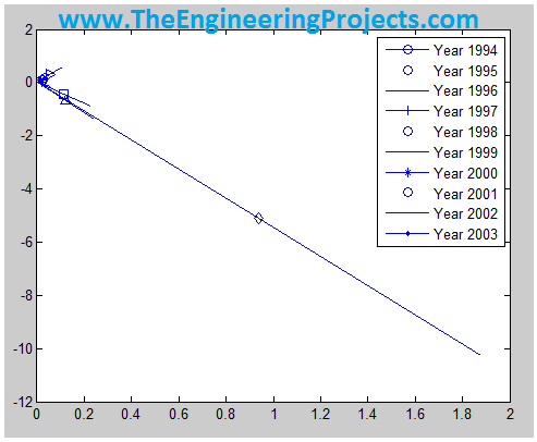
The original allocation figure is preserved above as a historical output. Its values are not presented as a new optimized portfolio or verified turnover record. Later in the tutorial, we will show the current Financial Toolbox methods that express the intended objective explicitly.
Step 7: Separate Forecasts From Backtested Returns
If mu is an estimated mean-return vector and w is a chosen allocation, muTw is an estimated portfolio return. Calculating that product from the same sample used for optimization is not a backtest. It tells us what the fitted model expects, not what subsequently happened.
A backtest needs a timeline. Estimate the model using information available up to a decision date, choose weights, then apply them to later realized returns. Repeat according to a stated rebalancing rule. Views used at each date must also have been available at that date.
% Illustrative one-period calculation with known beginning weights.
wStart = [0.50; 0.30; 0.20];
nextReturns = [0.02; -0.01; 0.005];
realizedReturn = nextReturns' * wStart; % 0.008, or 0.8%
The example gives 0.50 × 2% + 0.30 × -1% + 0.20 × 0.5% = 0.8% before costs. It uses future observations only to evaluate an already selected allocation. It does not use those observations to choose the same period's weights.
If you keep a constant weight vector for many periods and compute R*w on every row, you are implicitly rebalancing to those weights each period. A buy-and-hold portfolio instead allows weights to drift as asset values change. State which behaviour your calculation represents.
MathWorks provides a portfolio backtest framework with explicit strategies, rebalance rules and costs. A framework helps organize the process, but it does not prevent look-ahead bias if the supplied strategy uses future information.
Step 8: Calculate Portfolio Standard Deviation
Portfolio volatility is sqrt(wTSigma w). This includes both individual variances and cross-asset covariances. The original expression based only on squared asset volatilities and squared weights omitted the cross terms and is valid only under an additional zero-covariance assumption.
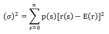
The historical formula image concerns variation around an expected return. For a multi-asset portfolio, we must apply the corresponding covariance calculation to the weighted combination, rather than treating every asset as independent.
SigmaExample = [0.0400 0.0060; 0.0060 0.0100];
wExample = [0.5; 0.5];
varianceExample = wExample' * SigmaExample * wExample;
volatilityExample = sqrt(varianceExample); % About 0.1245
For this hypothetical pair, the covariance terms raise variance from 0.0125 to 0.0155. The corresponding standard deviation is approximately 12.45%. A covariance matrix should be symmetric and positive semidefinite; substantial negative portfolio variance indicates an input or numerical problem, not a quantity to hide by taking an absolute value.
For realized monthly portfolio returns, sqrt(12)*std(rPortfolio) is a conventional annualization under appropriate assumptions about serial dependence. It is not the same as the volatility forecast made before the investment period, and it does not measure every form of risk.
Step 9: Estimate Alpha and Beta Consistently
A single-factor regression relates portfolio excess returns to benchmark excess returns: rp,t - rf,t = alpha + beta(rm,t - rf,t) + errort. Align all three series by date, currency and frequency before fitting it.

Beta describes the fitted sensitivity to the chosen benchmark. Alpha is the fitted intercept under that model. Neither coefficient proves skill or causality, and an apparently positive alpha may be statistically uncertain or sensitive to the selected benchmark.
% Inputs are aligned column vectors of realized monthly simple returns.
excessMarket = benchmarkMonthly(:) - riskFreeMonthly(:);
excessPortfolio = portfolioMonthly(:) - riskFreeMonthly(:);
assert(numel(excessMarket) == numel(excessPortfolio));
assert(all(isfinite(excessMarket)) && all(isfinite(excessPortfolio)));
mdl = fitlm(excessMarket, excessPortfolio);
alphaMonthly = mdl.Coefficients.Estimate(1);
beta = mdl.Coefficients.Estimate(2);
coefficientIntervals = coefCI(mdl);
This block requires your realized-return vectors and Statistics and Machine Learning Toolbox. The fitlm documentation describes the regression interface. Inspect residual behaviour and the assumptions behind its reported uncertainty; return observations may be heteroskedastic or serially dependent.
Do not combine a monthly intercept with an annual benchmark mean without a consistent conversion. Also, residual variance alone is not the complete covariance matrix of multiple assets. A factor model must include the common-factor contribution and its residual-covariance assumptions.
Step 10: Construct the Black–Litterman Prior
Black and Litterman's Global Portfolio Optimization describes an equilibrium starting point that can be adjusted using views. In a common mean-variance formulation, the implied expected excess-return vector is pi = delta × Sigma × wRef, where delta is a positive risk-aversion parameter.
This is reverse optimization. We start with reference weights and ask which excess returns are consistent with them under the selected covariance and objective. The reference might be a market portfolio or another documented baseline; it should not silently become whatever allocation looked best in hindsight.
The original article calculated an implied-return vector but did not complete the update with P, q and Omega. It also formed a covariance from weighted and percentage-scaled observations in a way that did not preserve the intended asset-return matrix. We will instead use an explicitly defined asset covariance throughout.
Choose Hypothetical Inputs
assetNames = {'Asset A','Asset B','Asset C'};
Sigma = [0.0400 0.0060 0.0080;
         0.0060 0.0225 0.0040;
         0.0080 0.0040 0.0625];
wRef = [0.50; 0.30; 0.20];
delta = 2.5;
tau = 0.05;
rf = 0.03;
pi = delta * Sigma * wRef;
C = tau * Sigma;
These assumptions imply annual excess returns of 5.85%, 2.6375% and 4.425% for A, B and C. They are calculated examples, not observations or recommendations. Adding the hypothetical 3% risk-free rate converts them into expected total returns under this convention.
C describes uncertainty about the prior expected-return vector. It is not the same as the covariance of realized asset returns. The scalar tau controls its size relative to Sigma in this formulation; calling tau a universal “precision” obscures its role. Smaller tau means a tighter prior when the other inputs are held fixed.
Represent Absolute and Relative Views
Let our first view be that A will outperform B by three percentage points, and our second view be that C will have a 6% excess return. The corresponding rows of P are [1, -1, 0] and [0, 0, 1]. The view vector q contains 0.03 and 0.06.
P = [1 -1 0;
     0  0 1];
q = [0.03; 0.06];
viewStd = [0.02; 0.03];
Omega = diag(viewStd.^2);
The second view is explicitly an excess-return view. With rf equal to 3%, it corresponds to a 9% total-return view. A relative view between two assets is unchanged by subtracting the same risk-free rate from both. This distinction prevents accidental three-percentage-point shifts in the input.
Omega expresses uncertainty about the views in squared return units. The diagonal example assumes independent view errors and uses standard deviations of two and three percentage points. It does not mean that we have assigned “2% confidence” and “3% confidence.”
Smaller uncertainty gives a view more influence relative to the prior. However, setting uncertainty to zero asserts an exact restriction and can create singular or inconsistent systems. Begin with finite positive uncertainties and examine sensitivity rather than using an extreme value to force a preferred allocation.
Calculate Posterior Returns and Uncertainty
Define A = P C PT + Omega. Then the posterior expected excess return is pi + C PTA-1(q - P pi). The expression q - P pi measures the difference between the stated views and the corresponding prior expectations.
The equivalent update is used in the MathWorks Black–Litterman code-generation example. In our implementation, matrix division solves the system without explicitly constructing its inverse.
assert(abs(sum(wRef)-1) < 1e-12);
assert(all(wRef >= 0));
assert(size(P,2) == numel(wRef));
assert(size(P,1) == numel(q));
[~, sigmaFlag] = chol(Sigma);
[~, omegaFlag] = chol(Omega);
assert(sigmaFlag == 0 && omegaFlag == 0);
A = P*C*P' + Omega;
muBL = pi + C*P'*(A \ (q-P*pi));
M = C - C*P'*(A \ (P*C));
M = (M+M')/2;
SigmaPredictive = Sigma + M;
muTotal = muBL + rf;
comparison = table(string(assetNames(:)), pi, muBL, muTotal, ...
    'VariableNames', {'Asset','PriorExcess','PosteriorExcess','PosteriorTotal'});
disp(comparison);
M is posterior uncertainty about the expected-return vector. Under the Bayesian predictive interpretation, the return covariance becomes Sigma + M. The MathWorks Financial Toolbox example explains this distinction. Some implementations keep Sigma for allocation instead; state which convention you use.
The symmetry adjustment removes tiny numerical asymmetry from floating-point operations. It is not a repair for an invalid covariance input. The Cholesky checks in this small example deliberately require positive-definite matrices; a more general semidefinite case needs appropriate numerical handling.
The original bar graph above displayed implied-return output. It is retained as a historical figure, not relabelled as the result of the new posterior calculation. To visualize the new example, plot pi and muBL side by side and identify both as hypothetical expected excess returns.
Optimize With the Posterior Inputs
We can now pass the posterior moments to a portfolio optimizer. The following continuation uses Financial Toolbox, the predictive covariance and long-only fully invested constraints. It chooses a maximum-Sharpe-ratio portfolio using the same hypothetical annual risk-free rate.
p = Portfolio('AssetList', assetNames, 'RiskFreeRate', rf);
p = setAssetMoments(p, muTotal, SigmaPredictive);
p = setDefaultConstraints(p);
wBL = estimateMaxSharpeRatio(p);
[riskBL, returnBL] = estimatePortMoments(p, wBL);
disp(table(string(assetNames(:)), wBL, ...
    'VariableNames', {'Asset','Weight'}));
If the objective is a target expected return instead, use estimateFrontierByReturn with a feasible target. Inspect the frontier endpoints first. An arbitrary 1% target may fall outside the relevant efficient-return range for the supplied assumptions.
Constraints can prevent the optimized weights from reproducing the unconstrained reference allocation exactly. Likewise, changing the covariance convention changes the optimization problem. Separate those effects from the effect of adding views when comparing allocations.
Evaluate Turnover and Realized Performance
Before a rebalance, compare target weights with the weights that actually exist after market movements. A common one-way turnover convention for fully invested portfolios is 0.5 × sum(abs(wTarget - wBefore)). The sum without the half measures total absolute weight traded under a different convention.
Costs depend on the amount bought and sold and the assumed execution conditions. A statement that turnover rises by a fixed percentage requires actual position records and a defined calculation. It cannot be concluded from a target-return number or an allocation chart alone.
When evaluating the strategy, compare it with the reference portfolio and a simple baseline under the same dates and cost rules. Report compounded return, realized volatility, drawdown and turnover separately. A strategy can improve one measure while worsening another.
Model Review and Sensitivity Checks
- Confirm that the no-view case returns the prior expected returns.
- Check that very uncertain views have little influence on the posterior mean.
- Change one view uncertainty at a time and inspect the resulting weights.
- Verify that every matrix follows the same asset order.
- Keep total and excess returns distinct at the optimizer boundary.
- Evaluate later observations without using them to create earlier views.
These are mathematical and experimental checks to apply to your implementation. A new execution of the historical commercial project is not claimed here. The supplied example is self-contained for the posterior calculation; its optimization and regression sections require their stated toolboxes and inputs.
Interpret Confidence Without Hiding Assumptions
The relative sizes of C and Omega determine how strongly the posterior moves toward the views. If both matrices are multiplied by the same positive constant, that scale cancels from the posterior-mean adjustment. The posterior uncertainty does still change. This explains why changing tau may appear to have no effect on the mean in implementations that also scale Omega proportionally.
In our example, Omega is specified independently from tau, so changing tau while holding Omega fixed changes the balance between prior and views. Document that choice before comparing results with another implementation. Two programs using the same tau can behave differently because their view-uncertainty conventions differ.
Correlated views also require attention. Suppose two views are derived from the same forecast and overlap heavily in asset exposure. Treating their errors as independent may count similar information twice. Off-diagonal entries in Omega can represent an explicitly justified relationship, but they must form a valid covariance matrix.
Do not create a view from the entire historical dataset and then pretend it was available at every earlier backtest date. That would turn a posterior calculation into a source of look-ahead bias. For a historical study, record when each forecast became available and how its uncertainty was estimated at that time.
Preserve a Reproducible Model Record
Save the asset labels, reference weights, covariance estimate, delta, tau, P, q, Omega and optimization constraints together. Include the return horizon, currency and whether each vector contains total or excess returns. A weight vector without that context is difficult to interpret and even harder to reproduce.
When reviewing a large allocation change, examine the view residual q - P*pi first. Then inspect the corresponding uncertainty and covariance links. A view about one asset can change several posterior returns because the model relates those assets. That effect is part of the calculation, but its magnitude should still be assessed against the assumptions that created it.
Frequently Asked Questions
Does Black–Litterman guarantee better returns?
No. It organizes assumptions about expected returns and uncertainty. Poor views, unsuitable covariance estimates or unrealistic constraints can still produce poor allocations.
Is pi the final Black–Litterman result?
No. It is the implied prior-return vector. The view update requires P, q and Omega, together with a stated prior-uncertainty model.
Can I average asset volatilities to get portfolio risk?
No. Use the full covariance expression. Correlation between assets is part of the portfolio's risk.
Why do my views not appear exactly in the posterior?
Finite uncertainty produces a blend with the prior. An exact match is not generally expected, especially when views conflict or share exposures.
Is multiplying estimated returns by weights a backtest?
No. A backtest applies previously determined weights to later realized observations under a documented trading and cost policy.