Hello friends! Today, we will work through financial calculations in MATLAB, beginning with historical market data and ending with portfolio risk-and-return plots. We will follow the original project's five stages: prepare the data, account for currency, calculate returns, estimate covariance and examine efficient portfolios.
The original project compared seven market indices and explored a 3% risk-free-rate assumption. We will retain that framework, but correct several important details about exchange rates, rolling windows and portfolio interpretation. An expected return is an estimate, not a guaranteed result, and a graph is only as meaningful as the inputs behind it.
This is an educational modelling example. The historical figures remain for context, while the formulas and code below explain a reproducible workflow. Information about the original commercial implementation is available on the project page; its old price and data-download dependencies are not assumed to remain current.
Step 1: Define the Data Before Downloading It
The earlier project used series identified by the provider symbols ^GSPC, ^NDX, ^GSPTSE, ^GDAXI, ^FCHI, ^FTAS and ^SSMI. These describe broad market or market-segment indices rather than seven equivalent industry sectors. Provider symbols and their availability should be checked when obtaining a new dataset.
| Project label | Market reference | Currency context to check |
|---|---|---|
| GSPC | S&P 500 | United States dollar |
| NDX | Nasdaq-100 | United States dollar |
| GSPTSE | S&P/TSX Composite | Canadian dollar |
| DAX | German equity market | Euro and historical-series conventions |
| CAC40 | French equity market | Euro and historical-series conventions |
| FTAS | FTSE All-Share | British pound |
| SSMI | Swiss Market Index | Swiss franc |
An index level is not a cash price for buying one unit of every constituent. It is a normalized measure with a provider-defined methodology. For an investable portfolio, specify the actual instruments or clearly state that the indices are research proxies.
Also distinguish price indices from total-return indices. A price series can omit dividends, while a total-return series includes a stated reinvestment treatment. Mixing the two creates a comparison that reflects data definitions as well as market performance. MathWorks discusses return inputs in its portfolio asset-moments documentation.
Replace Fragile Download Assumptions
The original code called hist_stock_data, which is not a standard MATLAB language function. A script using it requires that particular third-party implementation and a compatible data source. A historical example does not establish that its remote endpoint still works.
For a reproducible study, obtain data from a documented source and keep a local copy with its retrieval date, field definitions and adjustment policy. CSV or spreadsheet files can then be imported using MATLAB's table or timetable tools, including readtimetable.
Sort observations chronologically by their dates. Do not use flipud simply because one old provider returned newest observations first. Check duplicate dates, missing values and the common observation period before combining series into one matrix.
Step 2: Align Prices and Exchange Rates
Suppose Pt is a local-currency investment value and Xt is the number of US dollars per unit of that local currency. Its dollar value is PtXt. If the exchange-rate quote is instead local currency per US dollar, invert it before using this formula.
For an unhedged investment, the dollar simple return is:
1 + rUSD(t) = (1 + rLocal(t)) * (1 + rFX(t))For example, a 5% local return combined with a 2% increase in dollars per unit of local currency gives 1.05 × 1.02 - 1 = 0.071, or 7.1%. If that currency falls by 2%, the same local return gives 1.05 × 0.98 - 1 = 2.9%.
The original project multiplied every historical observation by one fixed exchange rate. That rescales the levels but leaves their percentage returns unchanged, because the constant cancels between consecutive observations. It therefore does not capture historical currency gains or losses.
When using total-return indices, multiplying by the dated exchange-rate series produces a proportional dollar-value series suitable for calculating dollar returns. Its absolute index level remains arbitrary. Normalize series for visual comparison if desired, but calculate returns consistently from their defined values.
Use Compatible Observation Dates
Choose a clear monthly sampling convention and align the exchange rate to the same valuation time as the investment value. Different markets close at different times, so a shared calendar date alone does not guarantee identical information timing.
Missing observations need an explicit policy. Forward-filling stale prices can create artificial zero returns and distort covariance. Dropping a row independently from one asset is worse, because it can place different months beside each other. Work from a common dated table and explain any exclusions.
Step 3: Calculate Returns in MATLAB
For simple returns, rt = Pt/Pt-1 - 1. For log returns, gt = log(Pt/Pt-1). Log returns add across time for a single investment, while simple returns combine directly across assets using beginning-of-period portfolio weights.
For the portfolio calculations here, we will use simple returns. The original code used differences of logarithmic levels, which is a legitimate quantity, but a weighted average of asset log returns is not generally the exact log return of the combined portfolio.
Prepare two CSV files with identical monthly rows and the same seven asset columns. Use a Month column in yyyy-MM-dd format, normalized to the same day convention. The first file contains positive local total-return levels; the second contains matching USD-per-local-currency rates, with ones in the US-dollar columns.
names = {'SSMI','FTAS','CAC40','DAX','GSPTSE','GSPC','NDX'};
prices = readtable('local_levels.csv', 'TextType', 'string');
fx = readtable('usd_per_local.csv', 'TextType', 'string');
if ~isdatetime(prices.Month)
    prices.Month = datetime(string(prices.Month), 'InputFormat', 'yyyy-MM-dd');
end
if ~isdatetime(fx.Month)
    fx.Month = datetime(string(fx.Month), 'InputFormat', 'yyyy-MM-dd');
end
assert(~any(ismissing(prices.Month)) && ~any(ismissing(fx.Month)));
prices = sortrows(prices, 'Month');
fx = sortrows(fx, 'Month');
assert(isequal(prices.Month, fx.Month), 'Dates must match exactly.');
assert(numel(unique(prices.Month)) == height(prices), 'Duplicate dates.');
monthId = year(prices.Month)*12 + month(prices.Month);
assert(all(diff(monthId) == 1), 'Monthly observations must be consecutive.');
P = prices{:, names};
X = fx{:, names};
assert(all(isfinite(P(:))) && all(P(:) > 0));
assert(all(isfinite(X(:))) && all(X(:) > 0));
assert(size(P,1) >= 3, 'More observations are required.');
usdLevels = P .* X;
R = usdLevels(2:end,:) ./ usdLevels(1:end-1,:) - 1;
returnDates = prices.Month(2:end);
This is a file-format contract, not a supplied market dataset. If your importer already produces datetime values in a different display format, configure its date import explicitly instead of forcing the illustrated conversion. Check a few rows by hand before applying the calculations to the full history.
Estimate Mean and Covariance
Rows of R are monthly observations, and columns are assets. The sample mean estimates the average return over the selected observations. The covariance matrix describes how asset returns vary together; its diagonal entries are variances.
muMonthly = mean(R, 1)';
SigmaMonthly = cov(R);
muAnnual = 12 * muMonthly;
SigmaAnnual = 12 * SigmaMonthly;
volAnnual = sqrt(diag(SigmaAnnual));
MATLAB's cov documentation specifies the observation arrangement and normalization options. The default sample covariance uses the sample correction. Keep that choice consistent when comparing results from different implementations.
Multiplying monthly mean returns and covariance by 12 is a conventional annualized moment approximation. Covariance scaling assumes an appropriate time-series structure, commonly no serial covariance. The annualized arithmetic mean is not the same as the realized compounded annual return.
For a realized sequence, cumulative growth is the product of (1 + rt). For example, +10% followed by -10% produces 1.10 × 0.90 - 1 = -1%, although the arithmetic average is zero. This is why a mean-return estimate should not be described as guaranteed growth.
Build Ten-Year Rolling Estimation Windows
Ten years of monthly returns means 120 return observations, requiring at least 121 price observations. The earlier index expression selected 132 returns per window, which is eleven years, despite the accompanying ten-year description.
Use explicit window lengths and derive the number of available windows from the data. With 240 monthly returns, a 120-month window moved forward by 12 months produces eleven windows. Fewer observations produce fewer windows; the code should not fabricate an extra year to match a legend.
windowMonths = 120;
stepMonths = 12;
assert(size(R,1) >= windowMonths, 'Insufficient history.');
starts = 1:stepMonths:(size(R,1)-windowMonths+1);
muWindows = cell(numel(starts),1);
covWindows = cell(numel(starts),1);
windowLabels = strings(numel(starts),1);
for k = 1:numel(starts)
    rows = starts(k):(starts(k)+windowMonths-1);
    sample = R(rows,:);
    muWindows{k} = 12*mean(sample,1)';
    covWindows{k} = 12*cov(sample);
    windowLabels(k) = string(returnDates(rows(end)), 'yyyy-MM');
end
These windows overlap heavily, so their estimates are not independent experiments. A series of similar frontiers can partly reflect shared observations. Label each curve by its estimation endpoint and preserve the start date in your analysis records.
Understand Portfolio Return and Risk
For a weight vector w and expected-return vector mu, the portfolio's expected simple return is wTmu. Its variance is wTSigma w, and its standard deviation is the square root of that value. The off-diagonal covariance terms are essential.
Consider two hypothetical assets with annual volatilities of 20% and 10%, a correlation of 0.3 and equal weights. Their covariance is 0.20 × 0.10 × 0.3 = 0.006. Portfolio variance is 0.25 × 0.04 + 0.25 × 0.01 + 2 × 0.5 × 0.5 × 0.006 = 0.0155.
The corresponding volatility is about 12.45%. Simply averaging the two volatilities would give 15%, while ignoring covariance would give about 11.18%. Neither is the correct calculation for these assumptions.
Step 4: Plot Efficient Frontiers
An efficient frontier contains portfolios that achieve the highest modelled expected return for a given risk level, subject to the chosen constraints. It is not created by drawing a straight line from the origin to one selected portfolio.
The following example requires Financial Toolbox. Its default portfolio constraints make weights nonnegative and require them to sum to one. Those assumptions exclude short positions and borrowing within the risky-asset allocation.
figure;
hold on;
for k = 1:numel(starts)
    p = Portfolio('AssetList', names);
    p = setAssetMoments(p, muWindows{k}, covWindows{k});
    p = setDefaultConstraints(p);
    W = estimateFrontier(p, 30);
    [risk, ret] = estimatePortMoments(p, W);
    plot(risk, ret, 'DisplayName', char(windowLabels(k)));
end
xlabel('Annualized standard deviation');
ylabel('Annualized expected return');
legend('show');
grid on;
MathWorks documents estimateFrontier and estimatePortMoments, including their argument and output order. Here, the first moment output is risk and the second is return. Swapping them would make the axis labels misleading.
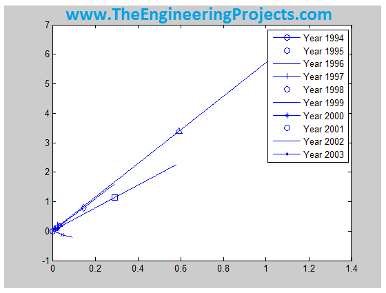
The original figure above is retained as a historical output. Its straight-line construction and earlier labels should not be treated as a newly verified set of efficient-frontier curves. Use the revised workflow to generate results from your documented dataset and constraints.
Step 5: Introduce a Risk-Free-Rate Assumption
A risk-free rate is a reference return for the chosen currency and horizon. It is not a “risk factor” that directly causes a business to lose money. Setting it to zero is an assumption, not an ideal world without investment risk.
We will retain 3% as a hypothetical annual input to explain the calculation. It is not a statement about a currently available rate. Keep its units consistent with the annualized expected returns and covariance used by the portfolio object.
rfAnnual = 0.03; % Illustrative assumption, not a current quote.
k = numel(starts);
p = Portfolio('AssetList', names, 'RiskFreeRate', rfAnnual);
p = setAssetMoments(p, muWindows{k}, covWindows{k});
p = setDefaultConstraints(p);
wT = estimateMaxSharpeRatio(p);
[sigmaT, muT] = estimatePortMoments(p, wT);
a = linspace(0,1,51);
lineRisk = a*sigmaT;
lineReturn = rfAnnual + a*(muT-rfAnnual);
figure;
plot(lineRisk, lineReturn);
xlabel('Annualized standard deviation');
ylabel('Annualized expected return');
grid on;
The maximum-Sharpe-ratio method selects a portfolio using expected excess return relative to risk under its assumptions. The line then combines that risky portfolio with the risk-free asset, with a from zero to one representing no borrowing.
The intercept must be rfAnnual. The old plotting expression used 0.02 at the intercept even when a different rate was selected. Extending the line beyond a = 1 would imply borrowing to increase risky exposure and would require additional assumptions about borrowing rates and feasibility.
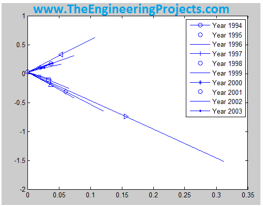
Changing the risk-free rate can change which risky portfolio maximizes the Sharpe ratio and the slope of its allocation line. It does not, by itself, change historical asset returns or prove that those assets generated losses. If the estimated risky returns do not offer a useful positive excess-return opportunity, inspect that result rather than forcing an attractive line.
Review the Model Before Interpreting Results
- Keep the same currency, return definition and time frequency throughout.
- Check that each covariance matrix is symmetric and numerically suitable for optimization.
- Inspect weights and constraints rather than only the final graph.
- Record the estimation dates, data source and adjustment rules.
- Separate in-sample estimates from later realized performance.
A covariance matrix estimated from too little data can be unstable or singular. Strongly overlapping indices can also create concentration that is less obvious from their names. Seven index series do not necessarily represent seven independent sources of risk.
For a backtest, estimate parameters using only information available before the investment period. Apply the resulting weights to later returns, account for the rebalancing rule and include relevant trading costs. Evaluating wTmu on the same estimated mean is an in-sample forecast, not an out-of-sample performance test.
Check Data Coverage and Historical Availability
The original download request ran from November 1993 to November 2013, a roughly twenty-year interval. That does not establish that every requested series supplied the same number of usable monthly observations. Check the actual first and last dates returned for each asset, rather than assuming the requested range was fully populated.
Historical currency treatment also needs care when a series spans a currency change. A provider may have rebased or back-calculated an index under a documented convention. Do not attach a modern currency label to every early observation without checking that convention. Your return calculation should follow the data definition, not merely the current country-to-currency mapping.
Keep a record of whether dividends are gross or net of an assumed withholding treatment, and whether the dataset is already currency-converted. Applying exchange rates twice or adding dividends to a total-return series would introduce a second adjustment that does not belong there. A clear data dictionary prevents these errors.
Distinguish Estimation Error From Optimizer Failure
An optimizer can correctly solve a problem whose inputs are poor estimates. If one asset receives almost all the weight, inspect its estimated mean, variance and covariance before blaming the solver. A small change in a noisy mean estimate can produce a large change in the selected portfolio.
Compare several reasonable estimation windows and report how much the weights change. This is a sensitivity exercise, not a reason to select whichever window happened to produce the best historical outcome. Choosing settings after inspecting all future results introduces information that would not have been available at the original decision date.
Constraints should express the intended portfolio rules. An upper bound on each position, a sector exposure limit and a turnover limit have different effects. Record them explicitly and avoid describing a constrained solution as the universal best portfolio. The result is optimal only for the particular objective, inputs and feasible set supplied to the solver.
Keep Fees and Compounding Visible
Suppose an illustrative strategy earns a gross monthly return of 1% and incurs a proportional cost of 0.2% of portfolio value at the start of that month. Its net growth factor is approximately (1 - 0.002) × (1 + 0.01) = 1.00798, giving a net return of 0.798%. State the timing convention rather than mixing a fee deduction into the return without explanation.
When reporting several months, compound the net growth factors. Do not add simple returns and label the sum as an exact cumulative return. Likewise, annualized volatility is a measure of variation under the chosen scaling assumptions; it is not a maximum possible loss or a confidence interval for future wealth.
A compact results table should therefore include the estimation period, constraints, expected return, estimated volatility and concentration, followed separately by any later realized return. Keeping forecasts and observations in different columns prevents a reader from mistaking an attractive model output for demonstrated investment performance.
Frequently Asked Questions
Can I use one exchange rate for the whole history?
It rescales levels but does not include currency returns. Use a dated exchange-rate series for an unhedged foreign-currency return calculation.
Does an expected return guarantee a profit?
No. It is a model input or estimate. Realized returns can differ substantially, including being negative.
Why do I need Financial Toolbox?
The matrix calculations use ordinary MATLAB functions, while the Portfolio class and frontier methods shown here require Financial Toolbox.
Are the old screenshots reproduced by this code?
No new reproduction is claimed. The code defines a corrected workflow requiring your prepared data files and installed toolbox.
What comes next?
Continue with the Black–Litterman approach in MATLAB, where we combine an equilibrium prior with explicitly defined views and distinguish estimated allocations from realized performance.