Mathematical Calculations in Ladder Logic

Hi friends, today we are going to explore mathematical computations in ladder logic. Like in any programing language you should find logic and mathematic computations, here in PLC programming you often need to process the input data that is collected from reading analog devices like temperature, level, flow et cetera. Then you need to run some calculations on this data to derive some other variables for deciding to run or stop some device or even to determine analog output to output to analog device i.e. valve or actuators. In the following sections, we are going to explore the mathematical functions and their input operators and outputs as well. Then we will show how to utilize such functions in ladder logic with simple examples and as usual enjoy practicing them thanks to the PLC simulator.

What are mathematical operations we have

You may find some minor changes in the set of mathematical functions from brand to brand of PLC controllers. However, you will find in most of them are common in every controller. For example, you will find the basic mathematical functions are available like addition, subtraction, multiplication, division, negation by applying two’s complement, modulus, increment and decrement, absolute, maximum, and minimum. In addition, trigonometric functions like sine, cosine, tangent are included. Let us go over these functions and explore their operators and output and how they can be utilized in PLC ladder logic programming.

Functions operators and outputs

For all these functions, they have input operators and one or more returned outputs. Most of them have two inputs like addition, subtraction, multiplication, and division. While some have only one input parameter like negating function, maximum, and minimum. And they all have only one input. Table 1 lists all these functions and their input operators and output.

Table 1: the functions’ input parameters and outputs


Operator and Output values data types

It is very important to be familiar with the type of data you are trying to process using these mathematical functions. So, simply you just need to know that the smallest size data type is a bool data type which is true or false or “1” or “0” and it uses only one single bit. Then character “char” or byte data type which is 8 bits while word data type is formed of 2 bytes or 16 bits and that is the word size in PLC. Also, there are doubleword data types that occupy 4 bytes or 32 bits. Moving to mathematical data types there are integer data types that can be stored in one word and the double integer “DINT” which can be stored in two words or 32 bit for holding numbers up to = 4294967296 for unsigned integers and half of that value for signed integers. Also, there is a real data type for holding numbers with floating-point. It needs 2 words or 32 bits and for a long real LREAL data type extends to 4 words or 64 bits.

How to use the mathematical function in ladder logic

In the TIA portal for siemens, there are two ways to add mathematical functions in a rung of ladder logic program. Figure 1 shows the first method which uses an empty box in the block interface and then you can select the function and its inputs and outputs parameters.

Fig. 1: Adding an empty box for including math functions

Figure 2 shows a list of functions from which you can choose the mathematical function you want to use.

Fig. 2: A list of math functions to select

Figure 3 shows another way to add a mathematical function by going to the basic instructions and then going over the math functions on the most right part of the window as shown and selecting the function you want to use.

Fig. 3: The second way to add a mathematical function

Figure 4 shows how to define the input and output parameters of the used mathematical function. For example, in figure two input parameters are defined as the function’s input operators which are literal number five and variable “x” which is predefined as an integer in the variable declaration section in the middle top section. Also, the Variable sum is defined as an integer. So the add function will add X to 5 and assign the result to variable Sum.

Fig. 4: Defining function parameters and outputs


Mathematical function ladder example

In this example, we are going to show how mathematical functions can be used in a ladder logic program and also show the simulation results. As in fig. 5, we design a simple calculator that uses the mathematical functions and each function can be triggered by a switch on a contact that is connected in series to the enable line of the function box.


Addition function math example

Figure 5 shows an additional example in ladder logic. It shows two operators A and B of integer data types. The variable A is located at address MW2 and variable B is located at address MW4 while the result is stored in variable RES which is located at address MW6. All of these variables are of type integer and size one word or 32 bits. The figure show simulation results on the PLC simulator and shows the RES variable holds summation of A and B.

Fig. 5: Addition function example


Subtraction math function example

Figure 6 shows a subtraction example in ladder logic. It shows two operators A and B of integer data types. The variable A is located at address MW2 and variable B is located at address MW4 while the result is stored in variable RES which is located at address MW6. All of these variables are of type integer and size one word or 32 bits. The figure shows simulation results before triggering the subtraction function on the PLC simulator. So, the RES variable holds zero before enabling the function.

Fig. 6: Subtraction function example not triggered

Figure 7 shows the simulation results after enabling the subtraction by switch or the “SUB” command contact. The Res variable now reflects the results of subtraction.

Fig. 7: Subtraction function example in ladder logic programming

Multiplication math example

Similarly, Fig. 8 shows an example for performing the multiplication process. First, the “MUL” is selected and two input operators of multiplications are given and output. The simulation result shows the RES variable holds the result of multiplication of the input operators.

Fig. 8: Multiplication function example in ladder logic programming


Division function example

Similarly, Fig. 9 shows an example for performing the Division process. The “DIV” is selected as an instruction to be executed and two input operators of division are provided and output. The simulation result shows the RES variable holds the result of the division of the input operators.

Fig. 9: Division function example after triggering


MOD function example

Similarly, Fig. 10 shows an example for performing the MOD function process. The MOD function determines the remainder of the division process, in this example we are dividing 25 by 10 which gives 2, and the remainder of 5. “MOD” function firstly is selected as an instruction to be executed and two input operators of MOD function are provided and output. The simulation result shows the RES variable holds the remainder of the division of the input operators.

Fig. 10: MOD function example in ladder logic programming

General calculation

Now, one may ask how I need to do the calculation in form of an equation that has many processes? This is a very smart question! Many programming tools support this, fortunately. For example, in Siemens, there is a function called “calculate” which can take two inputs and perform mathematical equations on these two variables and return the result in an output variable as shown in Fig. 11. It shows the function which is called “CALCULATE” and it has two inputs “IN1” and “IN2” and one output “OUT”. I triggered the help to show you an example that states OUT can be determined from the equation in inputs and also shows all functions that can be used including logic and mathematical functions. So we can use this function, in general, to act like any mathematical or logical function separately or by combining two or more functions in one equation.

Fig. 11: Using equations in ladder logic


Example of performing equation in Ladder logic

As you can see in the given example in fig. 12, the output variable can be determined based on multiplying the summation and subtraction of the input parameters as an equation. The result of the program is validated with a calculator.

Fig. 12: Using equations in ladder logic

Combining mathematical function

There is another way to perform combine many mathematical functions as shown in fig. 13. As you can notice, the output variable “out” can be determined by multiplying the summation of input variables “in1” and “in2” by “in1”.

Fig. 13: Combination mathematical function in ladder logic

Negate function

Negate function is one example of a single operator function in ladder logic programming. it reverses the sign of the input variable. For instance, fig. 14 shows an example of converting the sign of input variables “in1” to show the negative value reflected in the result in “res”.

Fig. 14: Single operator mathematical function in ladder logic programming

Absolute function

Figure 15 shows an example of getting the absolute of variable “RES” and saving it in variable “b”.

Fig. 15: Absolute function in ladder logic

Minimum and maximum in ladder logic

Getting minimum and maximum is one of the most frequently used in the mathematical operation. Figure 16 shows an example for getting a minimum of two input variables “in1” and “in2” while fig. 17 shows an instance of getting the maximum of two input variables as well.

Fig. 16: Getting a minimum of two input variables in ladder logic programming

Fig. 17: Getting a maximum of two input variables in ladder logic programming


Decrement and increment in ladder logic

One of the most commonly used functions is incrementing and decrementing one variable. For example, the counter variable all the time gets incremented and decremented through the logic of the program. Figure 18 shows an example for decrementing and incrementing an input variable. First, the initial value of the variable was 15, and then after incrementing it. The variable became 6 and then by applying decrementing operation it return to 5. It is very crucial to notice that, the user variable in increment and decrement operation works as input and output at the same time. Therefore, you can see in the increment and decrement blocks, it is defined as input-output “input”.

Fig. 18: Increment and decrement operation in ladder logic

Limiting variable in ladder logic

Now, let us use one of the very useful functions to secure a variable at specific limits. Figure 19 shows an example of limiting the value of one variable “in” to be sited between the specified minimum and maximum values. In that very example, the input variable has had a value of 5 and because it exceeds the set limit of maximum it is set to 4 which is the maximum allowed value to the variable thanks to the limit function.

Fig. 19: limiting variable in ladder logic programming

Trigonometric functions in ladder logic

Also, trigonometric functions like sine and cosine and other related functions can be executed in ladder logic. Figure 20 shows one example of how to use a sine function in ladder logic. The first rung in the example shows how to convert the degree into rad thanks to mathematical functions multiply and division. Ultimately, the sin function block is used to determine the sine of the given angle in rad.

Fig. 20: Triogonometrical function in ladder logic programming


What’s next

I am so happy that you be that patient to reach these points of tutorial and you know got familiar with most of the mathematical functions and how to use them flexibly through your program. The next round will go with the comparison operators and more deeply in mathematical logic flow using operators such as >,<,>=,<=, and ==. So please be ready for our next session of that ladder logic tutorial.

Interlock in Ladder Logic Programming

Hi friends and hope you are all very well. Today, we are going to deal with one of the most important and common problems that would be there in everyday tasks in industry and its solution. The problem is the safety of equipment and operators by preventing the machine from running under specific conditions for realizing the safety of equipment and human as well. Not only does it fulfill safety but also it is for performing the designed sequence of operation. If there is a problem, then it should be the solution for it. the solution is what so-called “Interlock”. So, what is interlock? And why do we need it? And how we can design a good interlock? Well! We may find such concerns exist in two aspects which are safety and operation sequence. In the first aspect, safety happens when we need to make the execution of one operation or process locked by some condition for realizing the safety of the operator or equipment. The second one is operation sequence for which we need to sort the operation into sequential and concurrent tasks according to the logic philosophy of the operation. That can be realized by preventing one task of execution until one other task is finished or letting one task wait until one or more conditions are fulfilled. I hope that makes the reason why we need interlock close comes to your mind. Now, how we can perform interlock? Well! It can be done in many approaches. However, we can say simply there is only and only one idea to do interlock. It is by putting the condition “contact” on which it will be decided if the process will go on or not, or based on it, one piece of equipment can go running or keep stopped. By completing this article, you will have known what is interlock, why we need it in industry daily life problems, its techniques, and for sure how to program interlock. Furthermore, types of interlock, real examples from industry, and how you can implement it using ladder logic programming in different ways will be ready for you to learn and practice in this tutorial.

What is interlock?

Interlock is how to prevent one process or equipment from running to satisfy safety requirements or fulfill the logic of the operation. A clear example of an interlock is to prevent cutting weapons from executing as long as the hands of the operator are away from the working area. In this case, there will be two push buttons on the left and right of the operator and out of the working space to make sure, when the operator requests the cutting machine to operate, his hands were pressing those two push buttons which are out of the working space. The previous example shows how to employ interlock for realizing safety purposes. Another instance that shows how Interlock can be used to satisfy the operation logic requirements is when we need to drive the motor in two directions. In that case, we commonly use two relays or contactors for forward and reverse directions. So, there should be an interlock of each contactor to each other meaning we cannot activate both at the same time because that will end up with a short circuit on the motor or the supply.

What are types of interlock?

There are two main types of interlock which are safety interlocks and machine or equipment interlocks. Safety interlocks for securing people from getting hurt while they operate the machine. And machine interlock concerns with securing the safety of machine parts and or realizing specific philosophy of logic. Figure 1 shows the different types and subcategories of interlock. The machine or equipment interlock can be classified into three types which are mechanical, electrical, and logical interlock types. And from their titles, the mechanical interlock can be physically satisfied by making mechanical connections between equipment to let or prevent them from running. An electrical interlock can be achieved by using electrical devices like relys’ coils, sensors, and switches. The first one which is relays’ coils is the most interesting electrical interlock technique as they can be utilized in creating a dependency between equipment so we can design flexibly dependence between two motors, for example, to not running simultaneously meaning one of two running scenarios. The last type is the logical interlock which is the most important here in this tutorial and I hope you get an astonishing start to master that type because that is the most frequently used in real life in the industry. Do you know why? Because it is done programmatically without the need for mechanical connections and setup or even electrical devices or hardwiring. Also, it is very flexible as you can change it when there is a need to change the logic at any time.

Fig.1: interlock types

Figure 2 shows the very example of a safety interlock to protect the operator from entering the zone of robot work to save him from the movable parts. Is that a mechanical or electrical interlock? Or maybe logical? What do you think? Well! Let’s move forward in the tutorial and come back to this question to see if you know the answer or not.

Fig. 2: the safety interlock

The non-safe interlock is designed for protecting equipment and lock specific processes from execution. The machinery interlock is classified into three main categories which are mechanical, electrical, and logic interlock. In mechanical interlock, a set of mechanical setups is designed to prevent equipment or operation from running at some operating conditions. Figure 3 shows a schematic of a mechanical interlock for a setup that makes the motor spin either forward or reverse direction and prevent enabling both at the same time. The dotted line represents the mechanical interlock between the two contactors for reverse and forward contactors for guaranteeing to enable only one of them at any given time.

Fig. 3 mechanical interlock example

Figure 4 shows the case of missing the mechanical interlock between the two contactors. It shows the possibility of activating bother of them at a given time. In that case, you can see the damaging effects on the motor and the short circuit possibility on the power lines.

Fig. 4: fault condition due to missing interlock

Another example of mechanical interlock is car steering interlock as shown in fig. 5. The steering wheel is interlocked mechanically and unlocked by inserting the key.

Fig. 5: car steering mechanical interlock

The mechanical interlock was commonly used in the past and my be exist nowadays but very rarely. On the other hand, the electrical interlock is the most commonly used in control systems currently. Similarly, the idea of electrical interlock can be achieved by preventing the flow of current between two devices at the same time. Typically two contactors or relays are used for achieving such electrical interlock. One of these contractors will be normally open and the other will be in a normally closed configuration as in Fig. 6. It is very clear that for energizing the lamp, CR2 will be energized when CR1 is de-energized.

Fig. 6: electrical interlock example 1

Another example of electrical interlock which is very common is the thermal overload shown in Fig 7. It shows two contactors are used in electrical interlock configuration. The main contractor is in a normally open configuration while the thermal overload contactor is in a normally closed configuration. When there the temperature is getting high to a specific value the thermal overload turns over from normally closed to normally open to disconnect the load.

Fig. 7: electrical interlock example 2

Now, let's move to the logical interlock which is our target in this tutorial. Logical interlock is applying the same concept of interlock programmatically. In this type, there is no mechanical or electrical physical connection for achieving interlock. Instead, programming is used to perform the interlock. This logical interlock saves the effort of commissioning including mechanical or electrical connections. In addition, it realizes reliability and flexibility.

Logical interlock in ladder logic programming

Figure 8 shows one example of logic interlock. You can notice the left part of the figure shows there are no mechanical or electrical hardwiring or connections between pumps 1 and 2. However, pump 2 is interlocked with pump 1 logically as shown in the most left part that shows the ladder logic code. To have pump 2 running, pump 1 should run first by the level switch. As shown on the right part of the figure below, when the level of the liquid reaches above the level switch, the switch is turned on and energized pump 1 which activates pump 2.

Fig. 8: logic interlock example 1

Figure 9 shows another logic interlock example in which a timer of type on delay is used to interlock equipment. As shown on the left the ladder logic code and on the right, an image shows the scenario of the logic with astonishing visualization. It shows that, when the operator presses the start pushbutton and keep pressing on it for the preset time value which is 3 second, the timer contact turns on and the coil of the contactor is energized. Now let us go to the lab and open our simulator to run those examples to validate their logic and verify their proper operations.

Fig. 9: logic interlock example 2

Logical interlock using ladder logic

Let’s get to experimental work, now open your simulator, the first example as shown in fig. 10, there are two pumps. And we need to run one pump at every given time. So, no one of them will work when the other does. The ladder logic code shown in Fig.1, uses the contact of each pump’s coil to lock the other pump. For instance, if the first pump is running, that will open the path to prevent energizing the second pump’s coil when it is requested to run. Similarly, the first pump’s coil is hindered from running while the second pump is running. It looks smart but let us test and see if the logic we designed matches the real-time environment or there is an issue to solve!

Fig. 10: The first example ladder logic program

Simulation example 1

Well! Now we have started our simulation. Figure 11 shows the initial case when no pumps are requested to run. So you can see each pump is all set to run once being requested.

Fig. 11: the initial case when no pumps were requested

Figure 12 shows the case when we requested the first pump to run. Because the stop button is not raised and the second pump is not running; The first pump goes running as shown in figure 12. So the question is that what is going to happen when requesting pump 2 to run?! Let’s see

Fig. 12: starting the first pump

Fig. 13 shows the case when we request pump 2 to run by hitting its start push button “start-pump2”. As expected, the second pump does not run for the interlock condition we designed for by putting a contact of the first pump’s coil as a condition to run the other pump. So let’s remove the hindering condition of interlock by stopping pump 1 and trying to run pump 2 and see.

Fig. 13: requesting one pump to run when the other is running

Figure 14 shows what happens when we remove the interlock condition. By hitting the stop push button of the first pump “stop-pump1”, the first pump has stopped. Consequently, the second pump went running once the interlock conditions has been removed. So now simulation verifies our design and proves our code of interlock is working great. Well done!

Fig. 14: remove the interlock condition by stopping the first pump

Interlock ladder logic example 2

As we aforementioned section earlier, the interlock could be done by sensors state or reading, running and stopping statuses of other equipment, or logical devices like timers or counters as well. Timers and counters can be used as an interlocking technique for creating a running condition based on some delay or specific counting. Figure 15 shows one example of a timer-based interlock in which the pump won’t run by hitting the start button until the operator holds the start push-button pressed for 3 seconds then the pump goes running.

Fig. 15: timer-based interlock ladder logic example

Figure 16 shows the simulation of the second example. My friends, please notice, despite the start pushbutton having been hit by the operator; the pump does not start because it waits for the timer to count 3 seconds, and then it can run.

Fig. 16: pump wait timer to start

Now after 3 seconds of holding start push-button pressed, fig. 17 shows the pump goes running because the interlock condition is no longer there. I am very happy you would get that!

Fig. 17: pump start running after 3 seconds

What’s next?

My friends, before talking about what we are going to practice next time; I just want to express my appreciation that you patiently follow up till this point and hope your experience moves forward and gets more and more every lesson. Next time we will navigate the mathematical functions and how to perform mathematical computations in your ladder logic programming. my friends I really can’t wait to see you very soon to practice mathematics in ladder logic programming.

How to use Counters in Ladder Logic Programming?

Hello friends! We hope you are very well! Today we are here for complementing our knowledge with one of the most important topics in PLC programming and practice its implementation in PLC ladder logic programming. Our topic today is about counters which help us to know the production size at any time, the repetition of specific tasks and events. Many real-life situation problems need counter like garage capacity should be tracked by using counters to report how many cars are inside and if there is room for incoming cars or it's full. Another critical problem is to count the repetitive tasks and events in manufacturing. Furthermore, counting products and pieces for taking an action like performing maintenance, stop operation, turn over to next production stage... et cetera.

Counter in conventional control

Counters are used in conventional or relay logic control. they mainly receive pulses and count these pulses and when it reaches a preset value the output coil of the counter is energized. They mostly include an LCD showing the counting as shown in figure 1.

Figure 1: Omron counter [1]

The main idea of most counters is counting input pulses by using logic circuits i.e. flip-flop and determining the output based on which an output relay is energized. There are two main types of the counter as regards structure: synchronous counters when all flip-flops and asynchronous counters when each flip-flop is connected to its separate clock. In addition, counters can be classified based on functionality into UP, DOWN, and UP-DOWN counters. If you are not familiar with logic circuit components like flip-flops so do not worry as it's not our concern here. We just want to let you know how physical counters in the traditional controller are complicated and take a lot of space as we need hundreds of flip-flops and other circuit components to have a counter which counts for a limited number. Figure 2 shows the logic circuit of the counter that can count from 0 to 9. It utilizes 4 flip-flops as shown. The type of this counter is an asynchronous counter as each flip-flop takes its clock from the output of the previous flip-flop. Furthermore, table 1 lists the truth table of the counter. It shows how the counter determines the count based on the output Q0, Q1, Q3, and Q4. For example, when all outputs are zeroes, that means the counter reads zero. When Q0 is high, Q1 is low, Q2 is low, and Q3 is high, that means the counter reads 9. But in PLC, it's the easier story, it’s software counters with flexible functionality and usability as well as we will see in the next section. So let's enjoy learning and practicing counters in ladder logic programming.

Figure 2: Asynchronous 0-9 counter

Table 1: the truth table of 0-9 counter

Pulse to be counted Q3 Q2 Q1 Q0
0 0 0 0 0
1 0 0 0 1
2 0 0 1 0
3 0 0 1 1
4 0 1 0 0
5 0 1 0 1
6 0 1 1 0
7 0 1 1 1
8 1 0 0 0
9 1 0 0 1
 

Counter in PLC

Simply, Counter in plc is an instruction to count up or down to preset value and energize an output at reaching that preset value. There are three types of counters in PLC which are:

Count up type

In this counter, each time a trigger input signal has been received at (CU), the counter counts up until reaching the preset value (PV) to energize output as shown in figure 3. The counter has three inputs: the trigger command, the reload command, and the preset value to set to what number the maximum counter is going to count up. Furthermore, it has two outputs: the counter output which is turned to true when the counter reaches the PV values, and the current value (CV) which tells the current value at any time to whom the counter reaches.

Figure 3: The counter Up instruction block [2]

Count down type

In this counter, each time a trigger input signal has been received at (CD), the counter counts down until it reaches zero at then the counter output is energized. As shown in figure 4, the counter has three inputs: the trigger command for counting down (CD), the reload command to reload to the PV value, and the preset value to set to what number the initial value from whom the counter starts the count down. Furthermore, it has two outputs: the counter output which is turned to true when the counter reaches the PV values, and the current value (CV) which tells the current value at any time to whom the counter reaches.

Figure 4: The counter down instruction block[2]

Up-Down counters

In this counter, the two functions of the count up and count down can be combined in one block. each rising edge of a trigger input signal has been received at (CD), the counter counts down. And each time it receives a command trigger signal at (CU), it counts up and so on till it reaches the PV values. At then the counter output is energized. As shown in figure 5, the counter has five inputs: the trigger command for counting down (CD), the trigger command for count up (CU), the reload command to reload to the PV value, the reset command to reset to zero, and the preset value to set to what number the initial value from whom the counter starts counting up or down. Furthermore, it has three outputs: the counter down output (QD) which is turned to true when the counter reaches zero, the counter up output (QU) which goes to true when the counter reaches the PV value, and the current value (CV) which tells the current value at any time to whom the counter reaches.

Figure 5: The counter Up-down instruction block[2]

Ladder program examples for counters

Now after we have introduced to counters in PLC as regard to their types, functionalities, inputs, and outputs, let’s get to have the fun of practicing our lab work for counters with our simulator.

Count up example

Figure 6 shows the ladder simple program example for a counter of type Up counter. In this example, the counter counts the input objects by a sensor that triggers the counter to increment. The ladder program is shown on the left side window while the simulator window appears on the right part. You can notice on the simulator window, we track all inputs and outputs as well. In the beginning, the current value (CV) is zero and the preset value is set to 10 meaning the counter will energize its output when it counts up to 10. Let’s press the input trigger and see what is going on. My friends, try to think before you go forward to see the simulator output as I am ganging will be the same as what you imagine!

Figure 6: Ladder example of a counter UP type

As you imagine exactly, figure 7 shows the counter is incrementing each time the input trigger signal is rising. Until it reach to or above 10 which is the PV value at then the counter output turns on as shown in figure 8.

Figure 7: The counter incrementing with triggering signal input

Figure 8: the counter output turns ON by reaching to or above the PV value

On the other hand, the reset signal can be used for resetting the counter to the zero to start over counting as shown in Figure 9.

Figure 9: the counter CV reset to zero by hitting the reset.

Count down example

This counter is used to count down from the PV value to zero. Figure 10 shows a very simple ladder program for the count down the program on the left part and its simulation appears on the right as well. The simulation windows show the PV value is set to 10 and the current value (CV) is initially starting from the PV value. Therefore, it starts with a value of 10. So let’s try to hit the input CD signal and see what the simulator shows.


Figure 10: Ladder example of count down counter

Figure 11 shows the counter is decrementing the CV by hitting the input CD. And continue decrementing until reaching zero. So what is going to happen then? Think!

Figure 11: the counter is decrementing by hitting the input CD

Exactly! And well though, as figure 12 shows, once the counter reaches zero, the output changes to true.

Figure 11: the counter output set to TRUE when reaching zero

Again, the reset button can be utilized to reset the counter to its initial state as shown in figure 12. You can notice that the CV reset to 10 which is the initial value and equal to the preset value (PV).

Figure 12: Reset button reinitiate the counter to the PV value

Count up-down example

Now we are going to combine all features in the UP and down counters in one counter which is called the UP-Down counter. Figure 13 shows a simple ladder example for that counter. The ladder code is shown on the left and the simulator window is on the right. The simulation window shows all inputs and outputs of the UP-DOWN counter.

Figure 13: A ladder example of UP-Down counter

Testing the up-down counter ladder program

We have two functions to test with this type of counter which is up counting and down counting. Figure 14 shows the initial state of the ladder program, it shows we start testing when the current value (CV) shows 2. So what do you expect when hitting the count up and the count down? Thinking and validate with the simulator results below.

Figure 14: initial state at the running of the up-down example

By hitting the count-up function, the counter acts like a UP counter and the current value is incremented as in figure 15.

Figure 15: count up function incremented the CV

On the other hand, by hitting the count down function, the counter acts as a down counter and the current value is decremented as in figure 16. And by pressing reset, the counter CV value will be reset to zero, while it reloaded to the PV value by pressing the load counter button. In addition, the output QU will be energized when the counter reaches or is higher than the PV value which is 10 in this example while the output QD will be true when the counter reaches zero. To sum up, this up-down counter can act as both types of counters UP and Down. I know someone is going to ask why we have such a counter when we already have one of each counter type? Well! That’s a really good question. And the answer is that, yes we can implement any problem relating to performing counting by using these two counters. However, some problems need to perform both functions UP and Down counting at the same time. For example, the Garage problem has cars getting in and out all the time and when cars get in we need to count up the cars and when cars get out we need to count down to report the number of cars in the garage at any time. So in such a problem, having one counter do the whole job is better than having two punters for reducing the conflictions and increasing the flexibility of calculations.

Figure 16: count down function decremented the CV

Next topic

I would like to thank you so much for following up with us up to this point of learning and practice. Despite briefly introducing the logic gates, we will elaborate in the next station on the logic gates and their functions and usage in ladder logic programming. So you be ready for more learning and practice the ladder logic and logic gates in deep detail.

How to Use Timers in Ladder Logic Programming?

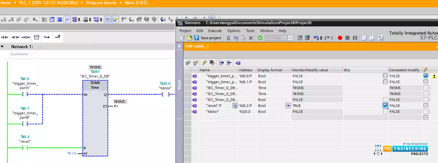
Hello friends! I hope you are doing very well, today we have a very crucial topic which is “timers”. Yes! Exactly like what comes to your mind. For running equipment i.e. motor at a specific time and/or for some amount of time we need timers. Timers are used even before PLC in classic or relay logic conventional control. However, there is a big difference between capabilities and limitations between using physical timers in classic or old fashion relay logic and using software timers in PLC. By completing this article you will be able to know what are timers and their types and applications. In addition, we are going to show off how to use timers in ladder logic programming with examples.

What are timers used for in industrial applications?

Well! This is a very good question to start and its answer can be taken as a motive to learn timers comprehensively. Timers are used to turn on actuators i.e. motors for a specific amount of time or turn off them after a specific amount of time. They are used for scheduling tasks on and off based on the process sequences.

How do timers work?

There are many types of timers based on the functions. However, all timers are working in the same principle that they are preset to a specific amount of time. Then when their coils are energized, the timers’ contacts are changing over to the opposite of their initial states i.e. from ON to OFF or from OFF to ON based on the delay time and the timer type. Therefore, we can imagine the main components of timers are the coil and contacts as shown in figure 1 [1]. It shows a relay timer for Telemecanique type showing the setting for the time delays, coil, and the contacts.

Figure 1: physical relay timer

Advantages of Timers in PLC over relay timers

The relay timers are limited in time setting i.e. for 24 hours and a specific amount of physical NO and NC contacts. While timers in PLC are logical software components with the unlimited setting of time which makes them very flexible with logic requirements. In addition, using physical relay timers costs us more space and wiring. While we can use soft timers in ladder logic with no limitations. Types of timers as we are going to describe in detail later, are limited to basic functions in the relay timers while all types of timers can be implemented in PLC using ladder logic programming.

Timers types

All timers have a coil and contacts and the latter will be changed over their states by energizing their coil based on the preset time and the type of timer. In the following subsection the most common timer types are introduced:

ON-DELAY timer

This type of timer is used to postpone the start of running. Figure 2 depicts the timing diagram of the On-Delay timer. As shown in this timer delayed the output from the input by the preset delay time. The figure shows that, after the input gets started, the time counts up until the preset amount of time elapsed, then the output starts as long as the input is ON. However, in the second pulse of the input, we can notice the output was not started because there was no chance to reach the amount of delay time that is preset in designing the timer.

Figure 2: The timing diagram of the On delay timer [2]

OFF-DELAY timer

In this type of timer, we aim at delaying the shutdown of the output. Figure 3 depicts the timing diagram of the OFF delay timer in which, the output starts at the time input starts and the output lasts after a specific time delay after the input gets off. You can notice that, in the second pulse of the input, the output did not shut down after the second pulse of the input due to the incoming of another input pulse before the delay time reached the preset value.

Figure 3: The timing diagram of the Off delay timer [2]

Pulse timer

This timer type energizes the output in each rising edge of the input for a fixed amount of time. Figure 4 shows the timing diagram of a pulse-type timer. It shows the output comes active each time it finds a rising edge of the input and keeps active for a fixed amount of time which is preset for the timer.

Figure 4: Timing diagram of, the pulse timer [2]


Accumulative timer

In an on-delay timer, if the input does not stay on for the preset time delay period there would not be a chance for the output to be energized. So there should be another modified timer to accumulate the period each time the input is ON and activate the output when reaching the preset value. This timer is called an accumulative timer and its timing diagram is depicted in figure 5. In this example, assume the preset values of 12 s, the first input pulse shown in blue resumes for 4 seconds and it goes on for another 8 seconds. The time is accumulated from the first and the second pulse until reached the preset value which is 12 seconds. The output gets ON as long as the preset time has reached and the input is ON.

Figure 5: on-delay accumulative timer

Timers in PLC and ladder logic program

Timers of different types can be used in PLC with great flexibility. Now let’s learn and practice timers with our simulator. But before we get to start we just need to introduce ourselves to the timer blocks in the ladder logic program.

Generate ON delay timer instruction

Figure 6 shows the instruction for generating an ON Delay timer. As you can see the instruction has two inputs and two outputs. The first input “IN” is the input contact of type Boolean. This input contact triggers the timer and initiates it to start counting the time. The second operand is the “PT” by which we set the required time delay. Moving to the outputs, the first output is “Q” this is the main output of the timer and it turns to true when the timer reaches the preset time delay. The second output is the “ET” which reports the time elapsed so far since the timer started to count time. The “PT” and “ET” are of time data type format and can be in milliseconds, seconds, minutes, hours, days et cetera.

Figure 6: Generate ON delay instruction

ON-Delay timer example ladder program

Figure 7 shows a very simple example program that uses an ON Delay timer for delaying the running of a motor. The ladder code is shown on the right part of figure 7. It shows that one input contact connected to address “I0.0” and its tag named “trigger_timer” is connected to the timer input. And the preset value is set to be one minute “T#1m” which means one minute. Notice the format is very simple. You type T denoting the time format and then “#” followed by the amount of time and at last the unit of time which could be “MS” for milliseconds, “S” for seconds, “m” for minutes, “d” for days … et cetera. Moving to the outputs, the timer output “Q” is connected to the motor meaning that the motor will be running after the timer counts complete one minute. The other output is “ET” which tells the time elapsed so far since the timer set to start counting time. Let’s go to the simulator window on the left side. We added all inputs and outputs to control the inputs and show the output as well. You can notice that, by setting the input “trigger_timer” to true, the timer starts counting the time as you can read in the “ET” variable that shows the time spent so far “T#29S_335MS” meaning 29 seconds and 335 milliseconds have been elapsed since input set to true. Since the PT time is not reached, the output is still false as shown in blue color.

Figure 7: ON-Delay timer sample program with a simulator

Figure 8 shows the moment when the timer reached the PT value which is one minute in our example. You can notice on the left window, the ET value becomes one minute which is equal to the PT value. Therefore, the timer output turned to true and the motor is switched on consequently. To sum up, this example shows how the output has become ON after one minute delay of the input.

Figure 8: ON-Delay timer energized the output after one minute delay

OFF delay timer example ladder program

After we have shown how we can delay the start of a motor by using the On Delay timer. Here we are going to show how to delay the shutdown. Figure 9 shows an example of a very simple ladder program that uses an OFF delay timer to delay the shutdown of an output. As you can see on the left the input is ON and the output starts running with the input at the same time. Let's try to set the input OFF as in figure 10, you can notice the output is still ON and the time counter is incrementing until it reaches the PT value which is set to one minute in our example. Figure 11 reports the moment at which the time counter reached the PT value which is one minute. At that moment the output or the motor is shut down. In a conclusion, the Off delay timer is our tool to delay the shutdown of output or terminate a process.

Figure 9: OFF delay timer example

Figure 10: The input is off while input is still run

Figure 11: the output shutdown delayed one minute

Pulse timer example

In this example, we are going to start and stop the motor in a pulsative operation mode thanks to the pulse timer type. That means the input to the timer will start the output to run for a specific amount of time that is present in the PT value regardless of receiving any other input pulses. In figure 12, the pulse timer example is shown. The very simple ladder logic program is displayed on the left window and the simulation is shown on the left window. You can notice that, once the timer received a high state of the input, it energized the output and started counting the time. However, when the input went OFF the output keep running ON for the designated while represented in PT value which is one minute for this example as shown in figure 13. Let’s test the condition of having another input signal as shown in figure 14. When the input goes again high which the last pulse does not complete, the output continues running and the timer does not reset its timing count. However, when the pulse time is reached as in figure 15, the output is shut down and the timer now is ready to start another pulse by noticing a rising edge of the input.

Figure 12: pulse timer example

Figure 13: the output continue running for its pulse period

Figure 14: another pulse does not reset the timer until complete one pulse period

Figure 15: output shutdown after completing pulse period

Accumulative timer ladder example

In this ladder example, we are going to show you how to continue accumulating the time until reaching the PS value at which the timer energizes its output as shown in figure 16. The example shows a very simple ladder code that has two inputs connected in parallel to OR logic. So any of these two inputs will trigger the counter to count up the time. On the left window, all inputs and outputs including timer operand and outputs are listed in simulating table to show the values while the program is executing.

Figure 16: an accumulative timer ladder example program

Let us start triggering the timer by one of the inputs as shown in figure 17. As you can notice the timer starts counting the time as shown in the ET value on the left window showing the simulation. What if we set the inputs OFF? In the ON Delay timer, the time will be reset. But in this timer, it does not and instead, it waits for another input signal to accumulatively increment the time till reaching the PT value as shown in figure 18. Let’s verify the concept by setting one of the inputs ON as shown in figure 19, the timer accumulates the timing counter until it reached the PT value which is set to one minute in this example. At that moment the output is energized as shown in figure 20. And finally, figure 21 shows how the timer is reset by switching on a reset button. One good practical example for using this type of timer is the maintenance schedule. For example, we can schedule the maintenance to be conducted after one year or after a specific amount of time or number of operating hours. So the timer will keep accumulating the time of operation regardless of the downtime and raise a flag to notify it is the time for performing maintenance.

Figure 17: starting the timer by enabling one of the inputs

Figure 18: setting the inputs off does not reset the timer

Figure 19: timer accumulates the time

Figure 20: the output goes ON after reaching the PT value

Figure 21: timer reset its timing count

What next

I would like to thank you so much for following up with our tutorial that far. So far you are familiar with timers types and how to utilize the suitable one for your task based on the logic you want to perform. Next tutorial we are going to go through counters showing their types and functionalities and for what reasons we need counters how we can use them appropriately.

Latching in Ladder Logic Programming

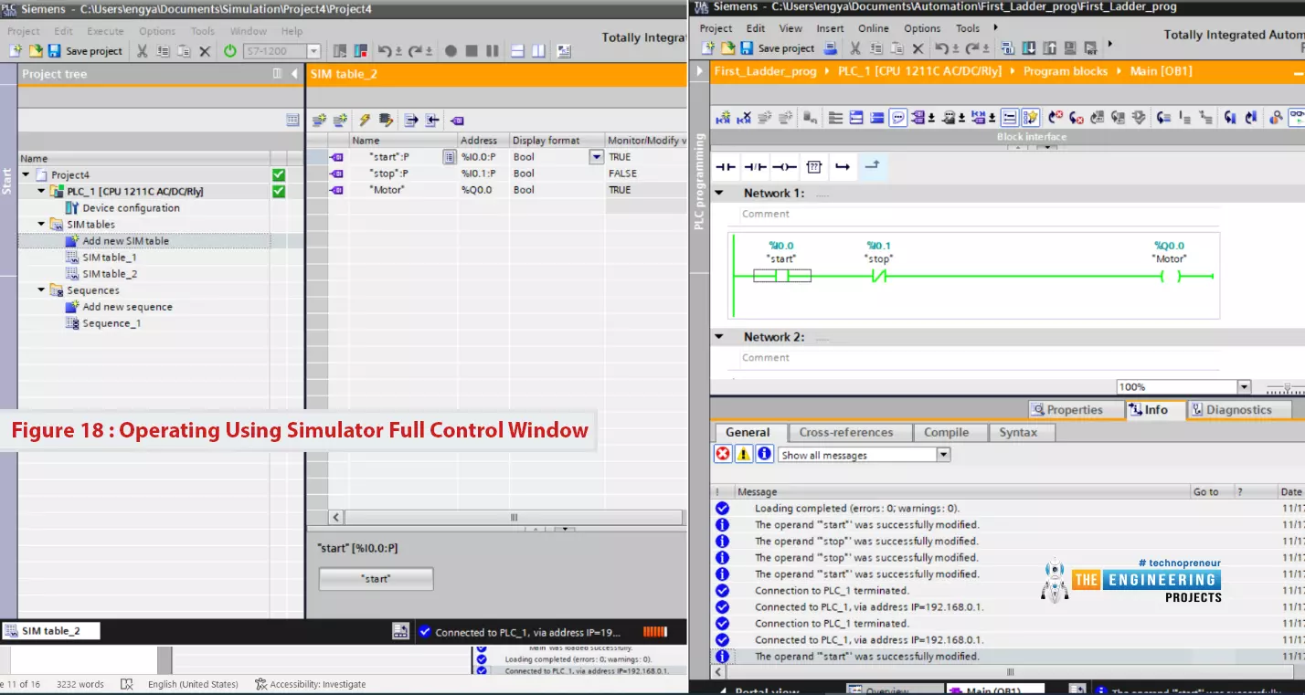
Hi friends! I hope you are doing well! Today we are going to learn and practice a new topic which is a very crucial technique in plc programming. the topic is called “latching”. We mean by Latching to keep the output running starting from the instance of giving a kick-off command until we hit a command to stop running of the motor. Imagine my friends, operator wants to start a motor by hitting a start push button and want the motor to keep running and leave and go for doing another task or job. And then it keeps running until the operator wants to stop it. The problem here is that, once the operator releases his hand away from the push button, the motor automatically stopped and that is not like what the operator wants to do with the motor. To clear the problem that we are going to solve, and for which we need to use the latching technique to connect a load, Figure 1 has been created for you to show the situation to make a direct connection to a motor by using a simple push-button. In this circuit, the operator needs to keep pressing the push button as long as he needs the motor to keep working. Otherwise, the motor will stop once he releases the push button. So would please think with to figure out what is the solution for that?

Fig. 1: Connecting motor to power by push button directly

Let’s try to connect the motor through a relay as it is typically in the industry. Maybe that helps us to control the way to energize the relay coil and use its contacts to start and stop the motor, Figure 2 shows how we can employ a relay to connect the motor to the power source. However, again In fig. 2, the operator still has to keep pressing the button as long as he wants the motor to keep running. This is not the best practice in real life, the operator has many jobs to do. So, he wants to give the command to commence running the motor and leave it running to perform some other tasks and then has the motor stops after the job has been done. In this case, latching is the best practice to connect the motor or any load we want it to run for a while or until complete some functions.

Fig. 2: relaying motor to DC power by hitting start push button

How does latching work?

Now, I hope you can feel the problem between our hands and sense the meaning of the word “latching”. Again, in a real-life situation, motors or any actuators can be run via relay, by energizing the relay’s coil, the contacts of the relay switches over from off to on and then connects the motor to let it starts spinning. So for running the motor, the rely on coil should be energized. However, the latching technique makes that requirements go away, instead of that, the contact that has been used for connecting the motor to power, is used to be another pathway to connect the rely on the coil to power without needing to keep pressing the start push button. WoW! What amazing solution is that! to just hit a button and then forget about it and use the contact to make like a closed-loop to have the coil connected to power forever and let the motor work forever. Ohhh!! Forever!!! How do we run the motor without stopping? Yes, you are correct. It should be a way to break that loop when we want to do stop it. we need a way to just stop the latching, to break its loop, to enable the operator to stop the motor when they need to do.

Steps to perform latching

Let’s now show you guys how we can establish and construct a complete latching circuit step by step. In the following subsections, three steps by which will be demonstrating how to complete a typical latching circuit including only push-button and relay.

Latching Step one

First of all, in a very simple circuitry which is shown in Fig. 3, the DC power lines positive and negative are connected with a push-button and relay to run a load. The positive wire in red is connected to the push button and then to the coil terminal A1 and A2, and then to the ground black wire. So now, it’s clear that when the push button is pressed it turned on and connects the circuit of the relay coil all the way to be energized. As a result, the contact of the relay is connected and now it is ready to connect the external circuit to run an actuator i.e. motor. But when the push button is released, the coil will be de-energized and the relay coil turns back to the open state and the motor is going to stop. So moving to the next step of building a latching circuit in which we aim at creating another pathway to supply the relay coil with power to forget about the push button and have it continue to run even after releasing the push button.

Fig. 3: the typical push-button and relay circuit

Latching step two

Now Fig. 4 shows the main wiring schematic of a basic latching circuit by which we indeed realize the concept and functionality of the latching technique. in the circuit, you can notice my friends that, the contact upper point and the relay upper point are connected in such a way that, it creates another pathway for energizing the relay coil without any needs to press or even touch the push-button B1. Again, when the push button B1 is pressed, the relay coil will be energized. As a result, the relay contact will be close contacted and in turn bridges point A1 to the positive red wire. Now, when the push button is released, the relay coil still has another pathway to connect to the positive wire so the relay coil will keep energized. I know now what comes out to your mind? if this configuration and schematic can put the relay coil in the loop and energize all the time by the first kick-off by hitting the start button thanks to the latching technique. The question now is, how about stopping the motor?. How to break this loop? Yes, that’s the only thing is remaining to complete a typical latching circuit.

Fig. 4: the second step of latching

Latching step three

We can name this step by ending latching. As shown in fig. 5, a normally close (NC) push-button B2 is added in the way from contact to the positive, red, power wire. Firstly, when the push button B1 is pressed, the relay coil is energized. And the contact of the coil is connected to the positive red wire as the push-button B2 is in a closed state by default. So now, it will be latching as long as the connection to the positive wire does not break. So by hitting push-button B2, it will turn out to open state and the connection to the positive wire is broken. Therefore, the relay coil will be de-energized and the latching gets to stop.

Fig. 5: Ending latching step 3

Latching in ladder logic programming

I know guys you all are waiting to come to this point to go to our lab and simulator and practice our tutorial. So now after we discussed the concept and basics of what latching is and how does it work? We now are all set to start our simulator and practice latching techniques in ladder logic programming as we used to do every tutorial.

Ladder logic without latching

Now we need to connect a simple start push button “input A” to the motor at “output” Q0.0 straight forward as in fig. 6. You can see, by pressing the input push button switch, the output motor starts spinning. But how about after releasing our hands off the start button?

Fig. 6: Before latching

Well done! Yes, exactly like what you expected, as shown in fig. 7, when the start pushbutton has been released, the motor stops immediately.

Fig. 7: the motor stops when we released the start button

Now by adding another pathway to run the motor as shown in Fig. 8, a contact from relay “output” has been used in parallel to form “OR” logic with the start push button. So, in the first place, when the start button is pressed, the output goes high and the closed contact now adds another pathway in “OR” logic.

Fig. 8: the latching effect in ladder logic example

Figure 9 shows how the closed contact that has been taken from the relay plays the role of the alternative path to connect the output to the power. So when the input start push button has been released, the closed contact of the output relay makes the connection and the output continue running. However, there is now one problem that, how to break that connection to stop the output?

Fig. 9: the latching effect after releasing the start button

The solution for having a way to shut down or break the latching connection is that, adding a normally closed (NC) push button “input B” in series as shown in fig. 10. This way enables to break the latching connection and shut down the output.

Fig. 10: adding a stop push button to end latching

So by hitting input B, the connection of latching is broken and the output stops running. But breaking the connection will make an issue if the input B is a switch like an emergency switch. The problem is that it should be returned to its normally closed state to enable the cycle to start by hitting input A or the start push button.

Fig. 11: the usage of adding stop button to end latching

By having the stop button return to the normally closed condition, the cycle can be restarted by pressing the start push button and enabling the latching once again.

Fig. 12: restarting the process by resetting the stop push button

Latching using set and reset

There is another way to perform latching of the output. The set instruction can be used to set the output to run until a reset command is met to reset the output. This is a piece of cake to latch an output by employing set and reset instructions. Let’s practice this way in the simulator. Figure 13 shows a simple ladder logic program that uses set and reset instructions to perform latching of the output. Input push-button input A is used to set the output while input push-button input B is used to reset the latch of the output.

Fig. 13: latching using set and reset technique

By hitting the input at I0.0 which is input A, the output is set to true. The question is what happens when input A becomes false?

Fig. 14: set to enable latching the output

Figure 15 answers our wondering that, even after input becomes false the output keeps energized thanks to using a set instruction. So when will see the output turns out to be false?

Fig. 15: the output keep set true even after input becomes false

After setting the output to true, it won’t become false until a reset command is used like in the example shown in fig. 16. The output is reset by input B and becomes a false state.

Fig. 16: reset to end the latching

What’s next?

I really would like to thank you guys so much to follow our tutorial till this point and I hope you have become well known for latching concepts, and how to use and utilize them to solve a real problem in real industrial life. Now let’s continue our series, learn and enjoy practicing ladder logic programming series. Our next station will be the comparator operators including equal, not equal, greater than, equal, less than, et cetera. And how to master using this operator to compare different data types and control the logic of a ladder logic program based on the results of these comparator operators.

Bottle Filling and Capping Project using PLC Ladder Logic

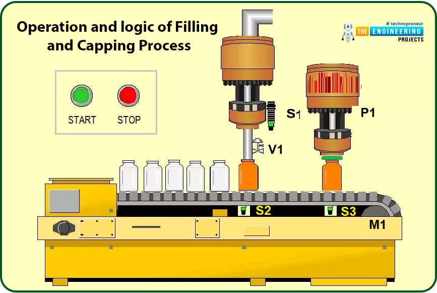
Hi friends, how are you doing? Today will integrate all of what we have learned so far in this series to build the first project based on ladder logic programming. Because we all are interested in industry, we pick one industrial project, Bottle Filling and Capping Projects, which is very common today. The problem we are going to solve today is bottle filling and capping. We have learned all basics of ladder logic including contacts and coils operation, logic gates, rising and falling edges, timers, and counters. So, today we will utilize all of these components to implement a complete ladder program of filling and capping problems.

Operation and Logic of Bottle Filling and Capping Process

For simplifying the operation of the process of filling and capping, fig. 1 shows the process flow which simply contains the main motor that drives the conveyor belt on which the bottles are running starting by hitting the start button. The conveyor belt starts running driven by motor M1 and the bottles move until sensor S2 detects one bottle, then motor M1 stops and the belt does so. At the same time, valve V1 opens to let water get dropped into the bottle until it reaches specific level thanks to level sensor S1. Then valve V1 closes and motor M1 goes on moving. Then when sensor S3 sees a bottle, the piston P1 is activated for capping the bottle and so on.

Fig. 1. The Filling and Capping Process

Process Inputs and Outputs

As you can see, for every single process in the industry, there are inputs and outputs. The inputs represent the sensors and user requests like starting and stopping the process. While the outputs are represented by actuators like motors, valves, and pistons. Table 1 lists the inputs and outputs of the filling and capping process. It shows the process consists of four inputs and three outputs including the function and description of each item.

Table 1: The list of Inputs and outputs of the Process

Logic Design of the Operation

Before going to ladder programming, we should design the logic of the operation to build guidelines on which we can develop the ladder logic. According to the operation description we stated aforementioned above, we can express the logic in lines as follows:

  • If start is ON, no filling is in progress meaning sensor S2 does not see a bottle, and no stop is requested, then motor M1 is ON.
  • If sensor S2 is ON, that means there is a bottle at a position to be filled so motor M1 will be stopped or OFF.
  • If sensor S2 is ON, that means a filling process is in progress, therefore, Valve V1 will open
  • If S1 is ON, that means the liquid in the bottle that is being filled reached the maximum level, So valve V1 closes and motor M1 now goes on running.
  • If S3 is ON, that means there is a bottle that presents at the capping station, So the piston P1 is retracted to process the capping of the bottle.

As you see in these few lines, we just wrote the philosophy of the filling and capping process’s logic. And the process keeps repeating until user requests stop. So now let’s move to convert this written logic into ladder logic rungs and enjoy for sure simulating the process in our lab to verify the logic we designed is correct or we need to amend.

Ladder Logic of Bottle Filling and Capping System

Before getting starting the filling and capping programming, we need to design the list of inputs and outputs of the program and their initial states. Table 2 shows a list of the inputs and outputs with their addresses and initial states.

Table 2: The Inputs and Outputs list with Addresses and Initial States

Figure 2 shows the first network in the designed ladder program. My friends, do not feel it a complicated because the fact is that, it is really simple. First of all, the start button to run the conveyor belt motor coil and latching is considered for letting the belt resumes running even after releasing the start button. Also, you should ask yourself during design two questions. The first is when the motor of the conveyor belt will be running and when to stop it? The answer to these two questions will end up with completing this network. For instance, the first question which inquiries about when to start the conveyor belt can show that the belt should be running by hitting the start push button to represent the request of the user to run the process. But, while the filling process is in progress marked by the activation of sensor S2, the conveyor should stop waiting for the filling process to complete by closing the valve when reaching the filling level limit noted by sensor S1. So, closing the valve is another signal that starts the conveyor once again. On the other hand, the conveyor belt should stop when the stop is requested by the operator in addition to sensor S2 that indicates a presence of a bottle in the filling station. So, you can notice two parallel branches to run the conveyor belt, one by start push button and one for latching. In addition, another parallel branch is added to run the belt by showing the completion of the filling process thanks to the signals of valve V1 status.

Fig. 2: Ladder Logic Network 1

Now, let’s have a look at the valve and ask ourselves the same question as what we have done with the motor of the conveyor belt (M1). what makes the valve V1 get closed and what causes it to open? For those causes to open the valve are the signal of sensor S1 that tells the bottle that is being filled is already filled and all set to move to cap station in addition to the latching consideration. So, we have two parallel branches, one branch for the sensor S1 and the other one from the valve status contact for latching. Those parrel branches connected in series to show “AND” logic with the sensor S2 to make sure of the presence of a bottle in the filling station. On the other hand, the stop push button represents an ending request received at any time from the user to close the valve.

Fig. 3: Ladder logic network 2

Now, the process goes on and the bottle has just left the filling station and has reached to capping station. That has been recognized thanks to sensor S3 that detects a bottle that has just arrived at the capping station. As a result, the piston should be activated. Firstly, a timer has been utilized to let the piston activated for some amount of time that is enough to let the capping process be comfortably completed. So, in-network 3 shown in fig. 4, a timer which is of off-delay type is utilized to activate the capping piston for plenty of time to let the capping process be completed as shown in fig. 5.

Fig. 4: Ladder Logic Network 3

Fig. 5: Ladder Logic Network 4

And finally, in-network 5 shown in fig.6, the falling edge signal of the piston denotes the completion of the capping process. So, a counter which is of type count-up timer is triggered to count up to determine the number of the processed bottle so far. The preset value has been set to a specific value i.e. 100 which can be used to perform maintenance or end a batch process for 100 bottles to be filled and capped.

Fig. 6: Ladder Logic Network 5

Compiling the Ladder Logic of the Project

After translating the writing logic to a ladder program that is composed of a couple of rungs, the second compulsory step is to verify the syntax of the ladder program and make sure that the program is free of error. So, we show you in fig. 7 the compilation results to show there is no error with the written code so far. By doing this verification, we are all set now to upload the program to the controller and check the logic and operations.


Fig. 7: Compiling the Designed Ladder Logic Program

Simulating and Testing

It is time to go to our lab and open the simulator to check the design and written ladder code. Figure 8 shows the initial state of the program before starting the process. It is clear that the conveyor belt is stopped and the status of all sensors, pushbuttons, actuators are as their aforementioned initial states.

Fig. 8: Initial State of the Inputs and Outputs Before Starting the Process

Now, let’s hit the start push button to start the process and watch what is going on. Figure 9 shows good news!!! By hitting the start button, the process correctly started and the motor M1 that drives the conveyor belt starts spinning. But, how about checking to release the start pushbutton by leaving our hand to see what’s going on?

Fig. 9: The status After Hitting Start the Process

WoW!!, well done, latching is working as shown in fig. 10 as the conveyor continues spinning even after releasing the start button thanks to applying the latching technique.

Fig. 10: Conveyor Still Running Even after Release start Push Button Thanks to Latching

Once a bottle is presented at the filling station, sensor S2 is activated. Consequently, the conveyor stops waiting for the filling process to complete. But, when does the filling process ended and how to know it’s done already to go further?

Fig. 11: Conveyor Stops when a Bottle Presents at S2 for Filling

Well! Sensor S1 is there to watch the level to which the liquid reaches in the bottle that is being filled. Once the limit is reached, sensor S1 is activated telling hey here we go, the filling process is over and now we ready to go further to the next step which is the capping station as shown in fig. 12.

Fig. 12: The Valve is Closed by reaching the Limit Level and S1 is ON

Because the valve is closed after the filling limit is reached, the conveyor continues spinning and sensor S2 is deactivated showing the bottle has been filled and left the filling station. However, the conveyor belt keeps running thanks to the latch again as shown in Fig. 12.

Fig. 13: The Conveyor belt Goes Running by Closing The Valve V1

Let’s now my friends check what’s happening by reaching the capping station? Astonishing !!! as we put there our agent to tell us a bottle has arrived for capping which is sensor S3, once that happened, sensor S3 is activated and hence activates the piston to retract and keep retracted for a sufficient amount of time to let the capping process be completed thanks to using a timer of type off-delay timer. So first fig. 14 shows in network number 3, the timer is activated and starts counting the time that is preset to 2 seconds and in the same time activates the piston to keep retracted during that time based on the nature of operation of an off-delay timer.

Fig. 14: The Piston is Activated by Reaching at Capping station When S3 is ON

And finally, the counter is utilized to count the processed bottles which are triggered by the falling edge of the piston denoting completion of a filling and capping process.

Fig. 15: The Counter Counts up Every item After the Capping Process

What’s next

By reaching this line in our tutorial, I would like to congratulate you that you are now all set to think about complete basic problems in the industry and design the logic to solve them and write the ladder code. Is here the end station of our ladder logic tutorial? For sure no, we still have a lot to move forward from the basic level to become experts. So wait for the next tutorial in which we go deeply into details of math and logic functions and data processing.

Signal Edge Detection in Ladder Logic

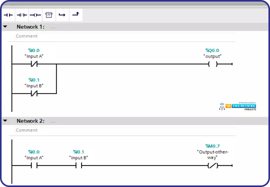
Hello friends, How are you doing? Today, we have a very interesting topic of PLC ladder programming which is how to detect the transition between true and false and from low to high?. I know you are asking why do we need that? Well! Imagine my friends, we want to start a motor when the input signal state changes from high to low or from false to true. Let us give two examples to highlight the edge detection techniques. Good examples of using edge detection-based logic are timers and counters. In counters, they are energized to count up or down when a signal appears and the same for timers. Figure 1 shows the difference between using the edge to control a motor. In the top part, the motor is controlled by an input switch. the output is ON and OFF based on the status of the input. But, in the second example, the rising edge is used to energize a motor. So, the motor comes to true when the switch state changes from false to true. On the other hand, imagine my friends if you want to activate a protection relay or safety function based on the result of the logic operation (RLO) for output, in that case, we can control the running of the output for one scan cycle to be based on the change in the state of the RLO.

Fig. 1: Rising edge logic

Signal Edge Types

There are two edge types:

  1. Falling edge.
  2. Rising edge.
Figure 2 shows the falling and rising edge signal. It shows the falling edge happens when the signal turned from true to false while the rising edge when it signals changes from false to true.

Fig. 2: The falling and rising edge of a signal

Rising Edge in PLC Ladder Logic

Figure 3 shows the general symbol of a rising edge. The letter “P” denotes a positive edge. while fig. 4. Depicts the rising edge in ladder logic in the TIA portal of siemens software.

Fig. 3: the general symbol of a positive or rising edge

In ladder programming, the rising edge shows a positive rising edge received for the signals. In fig. 4, the rising edge is for the signal tagged as “TagIn_4” and the previously saved value is stored in “Tag_M”. the system can recognize a rising edge by comparing the buffered value stored in “Tag_M” and the current value in “TagIn_4”. For example, if the previous value stored in “Tag_M” is False, and the current value in “TagIn_4” shows high logic, this would mean a rising edge is received.

Fig. 4: the rising edge in a plc ladder program

Falling edge in PLC ladder

Figure 5 shows the general symbol of a falling edge. The letter “N” denotes a negative edge. while fig. 6. Depicts the falling edge in ladder logic in the TIA portal of siemens software.

Fig. 5: the general symbol of a negative or falling edge

In ladder programming, the rising edge shows a negative or falling edge received for the signals. In fig. 6, the falling edge is for the signal tagged as “TagIn_4” and the previously saved value is stored in “Tag_M”. the system can recognize a falling edge by comparing the buffered value stored in “Tag_M” and the current value in “TagIn_4”. For example, if the previous value stored in “Tag_M” is True, and the current value in “TagIn_4” shows low or false logic, this would mean a falling edge is received.

Fig. 6: the falling edge in a plc ladder program

Set Output on a Positive Edge

Now let’s do the same concept on the output side, fig. 7 shows the set output ladder instruction on a rising or positive edge. In this instruction, the result of the logic operation (RLO) which represents the left part before the output is evaluated to check the transition in its state. If the RLO changes from false to true then the output will be set for one scan cycle.

Fig. 7: the set output on positive edge instruction

Figure 8 shows an example of the set output on a positive edge. On the most left, the coil with the letter “P” inside represents the instruction. The instruction works by saving the previous value of RLO into “Tag_M” and verifying the changes in a state with “TagOut”. For example, if the “Tag_M” holds a true state while the previously stored value in “Tag_M” was false. That would show a positive edge and the output will be set to true for the complete scan cycle.

Fig. 8: example of set output on a rising edge

Set Output on a Negative Edge

Figure 9 shows the set output ladder instruction on a falling or negative edge. In this instruction, the result of the logic operation (RLO) which represents the left part before the output is evaluated to check the transition in its state. If the RLO changes from true to false then the output will be set for one scan cycle based on detecting a falling edge of RLO.

Fig. 9: instruction of set output on falling edge

Figure 10 shows an example of the set output on a falling or negative edge. On the most left, the coil with the letter “N” inside represents the instruction. The instruction works by saving the previous value of RLO into “Tag_M” and verifying the changes in a state with “TagOut”. For example, if the “Tag_M” holds a false state while the previously stored value in “Tag_M” was true. That would show a negative or falling edge of the RLO. Consequently, the output will be set to true for the complete scan cycle.

Fig. 10: example of set output instruction base don falling edge

Simulating edge detection

Now let’s go to our lab and open a simulator to enjoy practicing very critical points in ladder logic programming. Yes, my friends, these are very critical points and are used smartly in solving very hard problems to solve. But, by comprehensive these points, you will be superb in your field as a prospective ladder logic programmer. Two points we are going to simulate, the first one is the ringing and falling edge of the inputs and their effects on activating and energizing the output for a complete pulse. And the rising and falling edge cases of the result of logic output (RLO) and its effects on energizing the output for a complete pulse.

Simulating rising edge

Now, let’s assume we have a situation in the factory that, when specific action occurred, the output will be energized. In the example represented by fig. 11, when and only when input A, turned on, we need to start the output. That means the only scenario in which the output is turned on is when input A state changed from false to true. So let us simulate three scenarios, the first one shown in fig. 11, in this scenario the input previous status is saved in input B, while the current or new state is saved in input A. notice when the input does not change and it is false, the output is turned off.

Fig. 11: the rising edge scenario 1

Now let’s turn on input A, so now input changed from false to true as shown in Fig. 12. Ohh, notice the output comes true and that’s the rising edge at when the input changes from false to true.

Fig. 12: the rising edge scenario 2

And in the last scenario, when the input keeps true meaning the previous status was true and the current state is true, then the output is false as shown in Fig. 13.

Fig. 13: the rising edge scenario 3

In a conclusion, in rising edge, the output only gets true when the input changed from false to true.

Falling Edge in PLC Simulator

Now, let’s assume we have another situation in the factory that, when an input or sensor turns off or changed from true to false, the output will be energized. In the example represented by fig. 14, when and only when input A, turned out from ON to off, the output will be energized. That means the only scenario in which the output is turned on is when input A state changed from true to false. So let us simulate three scenarios, the first one shown in fig. 14, in this scenario the input previous status is saved in input B, while the current or new state is saved in input A. notice when the input does not change and it is false, the output is turned off.

Fig. 14: the falling edge scenario 1

Now let’s turn on input A, so now input changed from false to true as shown in Fig. 15. Ohh, notice the output is false because that’s not a falling edge as the input changes from false to true.

Fig. 15: the falling edge scenario 2

And in the last scenario, when the input changed from true to false which is a falling edge. Therefore, the output turned on as in fig. 16.

Fig. 16: the falling edge scenario 3

In a conclusion, in a falling edge, the output only gets true when the input changed from true to false.

Simulating set output on the rising edge

Now, my friends, we need to run the output for one pulse based on the result of logic output (RLO). Figure 17 shows the scenario of having a false state of the RLO, the output is false because there is no falling edge detected for the RLO.

Fig. 17: set output on rising edge scenario 1

Figure 18 shows the case when the RLO is turned from false to true, the output comes true but for one pulse notice the previous status represented by buffer has become false but the output after pulse time returns to false. However, the pulse of the output has been detected thanks to energizing output tag_5.

Fig. 18: set output on rising edge scenario 2

Simulating set output on falling edge

Figure 19 shows the very initial case of set output with a falling edge. To show, the case of the falling edge of RLO, we use another rung that would energize another output at Q0.6 when and only when the falling edge of the RLO occurs. In Fig. 19, the RLO was false. Therefore, there is no cause for a falling edge when RLO changed from true to false. So the output shows a false state.

Fig. 19: set output on falling edge when RLO was initially false

Now let’s turn on the RLO, so the RLO changed from false to true which is still not a case of a falling edge of the RLO. SO the output is still false as shown in Fig. 20 represented by output Q0.6.

Fig. 20: set output on falling edge when RLO turned to on

Figure .21 shows the scenario of the RLO turning from true to false which is a falling edge. In that case, the output will be turned on for one pulse and as a result, latching output at Q0.6 as shown in rung 2 of fig. 21.

Fig. 21: set output on falling edge when the RLO turned back to false (falling edge)

What’s Next

Once more I would like to thank all my friends for continuing with our learning and practicing our PLC ladder logic series. Now we have learned the concept of edge detection, its importance, and how we can utilize the rising and following edge in some critical and accurate cases of logic. The rising and falling edge of the inputs can energize an output in a pulsative way or for only one pulse. This scenario exists in the industry and is very common. For example, when you want to energize a safety device by the occurrence of some conditions like increase of liquid level or temperature or pressure et cetera. Also, the result of logic output (RLO), can be used to set or reset output for one pulse. In the next tutorial, we are going to introduce the latching in more detail showing why we need to latch an output, the ways of latching with examples, and for sure enjoying our practicing with the PLC ladder logic simulator.

Simulating Advanced Logic Gates using Ladder Logic Programming

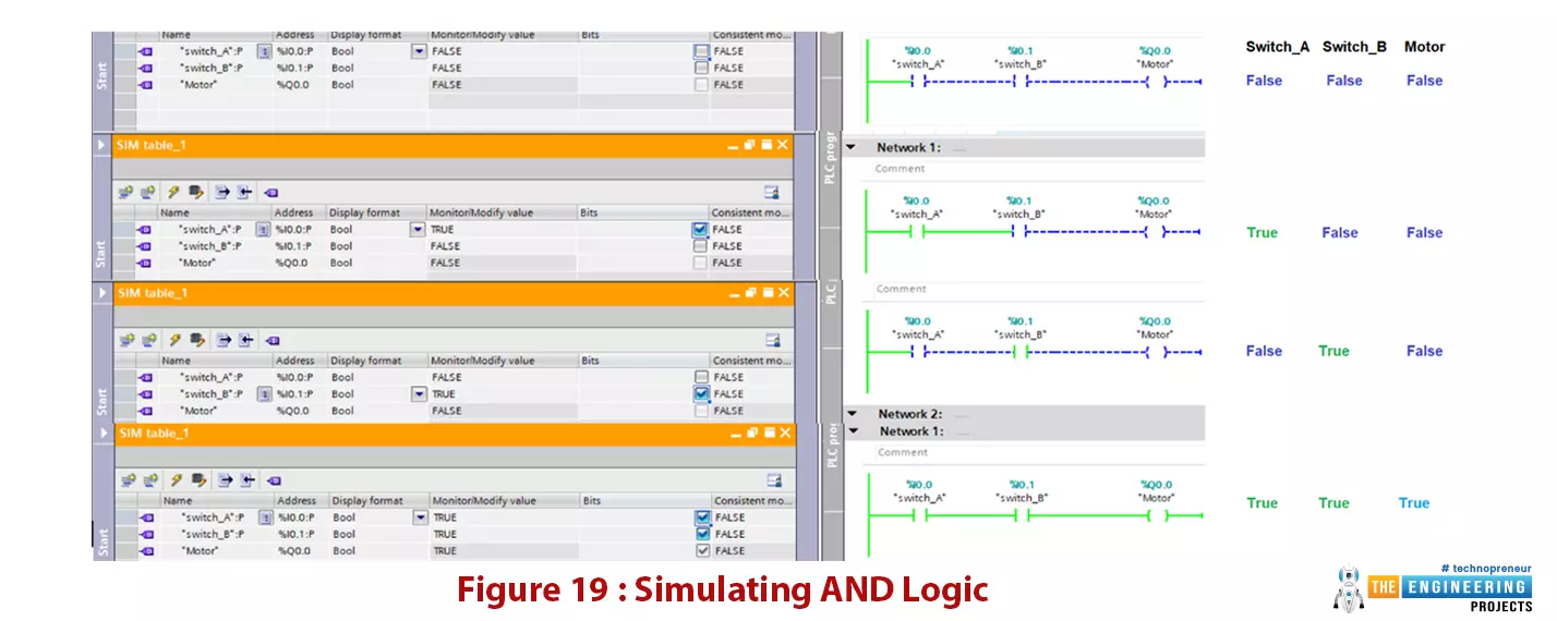
Hello friends! I hope you are all very well! I am so happy to meet you today to continue learning and practicing PLC ladder logic programming. In an earlier part, we already have gone through the very basic logic gates of “AND”. “OR”, and “NOT”. Today we are going to resume the simulation of logic gates. We have started and gone through simulating the basic logic gates which are “AND”, “OR”, and “NOT” as they are the most important basic logic gates by which we can form other logic gates. However, because the logic of large-scale projects is getting more and more complicating, a lot of time we have to use the other functions to do tasks faster. For example, we have shown in the logic gates article that, XOR can be used to compare two inputs and check if they are equal or not. On the other hand, someone may say, oh we can do XOR by using the basic three gates of “AND”, “OR”, and “NOT”. That’s correct. So why do we need to go learning other logic gates when we can implement them by using that three basic logic gates. Well! That is a very good question.

Working in ladder logic programs is getting further complicated especially for large-scale projects. So, it is very beneficial to know shortcuts for writing ladder logic simpler, more readable, and easier for others to develop. Using this variety of logic gates, enrich the logic and fluency of writing the logic in different situations. For example, using XOR logic is very common for comparing two inputs to decide if they are equal or different. Therefore, we found that it is crucial to go through all logic gates and do simulations for them all in this tutorial. for coherently we get the knowledge to use them fluently in ladder logic programming to solve different logical problems and scenarios. There are seven basic logic gates which are: “AND”, “OR”, “NOT”, “NAND”, “NOR”, “XOR”, and “XNOR”. We have gone through “AND”, “OR”, and “NOT” logic gates including simulation work. So let us go through the other four gates for learning and practicing all basic logic gates.

The "NAND" Logic Gate

The “NAND” logic gate is the invert of the “AND” gate like you invert the output of an “AND” logic gate as shown in Fig. 12. Table 5 lists all combinations of the inputs and the output of the “NAND” logic gate.

Fig. 12: NAND symbol

Table 5: the truth table of the “NAND” logic gate

Input A Input B Output
0 0 1
0 1 1
1 0 1
1 1 0
 

In addition, the timing diagram of a “NAND” logic gate is shown in fig. 13, it shows the output goes low when both of the inputs A and B are true which is the inverse of the “AND” logic gate. Also, Fig. 14 shows a ladder logic of a “NAND” logic.

Fig. 13: The timing diagram of the “NAND” logic gate

Fig. 14: Ladder logic sample of a “NAND” logic

NAND Logic in PLC simulator

The NAND logic gate can be considered as the invert of the “AND” logic gate. So as listed in table 1, the truth table of AND and NAND logic gates shows how the NAND gate is the reverse of the AND gate. Also, it shows the NAND gate should come out to your mind when you want the output always low except when both inputs A and B are high.

Table 1: the truth table of the AND versus NAND logic gate

The NAND gate can be implemented by connecting the negate of the output in series to the inputs A and B. Another way to implement NAND is by inverting both inputs and connecting them in parallel as shown in fig. 1. Rung 1 and rung 2 respectively.

Fig. 1: The NAND ladder logic in two ways


Let’s test our ladder logic in both methods. According to the truth table of NAND gate, we have four test cases. figure 2 shows the first test case when both inputs A and B are false. In this case, the output should be true as shown in fig. 1.

Fig. 2: NAND ladder logic when both inputs are false

figure 3 shows the second test case when inputs A goes true while B is false. In this case, the output should be true as shown in fig. 3.

Fig. 3: NAND ladder logic when input A is false and input B is true

Figure 4 shows the third test case when inputs B goes high while B is low. In this case, the output should be true as shown in fig. 4.

Fig. 4: NAND ladder logic when input A is true and input B is false

Figure 5 shows the last test case when both inputs A and B become high so the output goes false as shown in fig. 5.

Fig. 5: NAND ladder logic when both inputs are true

Thanks to performing the simulation of the NAND gate, we now can conclude that we should be looking for a NAND logic when we want to shut down an actuator i.e. motor whenever two inputs are in a true logical state simultaneously. For a practical example, when we have three pumps and we want to run them in the mode of two of three. There should be only two of the three pumps to run at any time. In that case scenario, the run condition of any motor can be a NAND of the status of the other two motors.

The “NOR” Logic Gate

The “NOR” logic gate receives two inputs and has one output. It is the same as the invert of the “OR” logic gate. Like you follow the output of an “OR” gate by a “NOT” logic gate. Fig. 15 shows the symbol of a “NOR” gate. In addition, the truth table is expressed in table 6. It shows the output becomes false only when one of the input A or input B or both goes high which is the reverse logic of the “OR” logic gate.

Fig. 15: The symbol of “NOR” gate

The “NOR” logic gate can be formed by connecting the “OR” logic gate to the inverter “NOT” logic gate. Or by inverting the inputs by using “NOT” logic gates and connecting them to the “AND” logic gate as shown in Fig. 16.

Fig. 16: structure of “NOR” logic gate

Table 6: the truth table of the “NOR” gate

Input A Input B Output
0 0 1
0 1 0
1 0 0
1 1 0
 

Figure 17 shows an example of a ladder program for implementing the “NOR” logic gate. It shows that the “NOR” gate can be implemented in ladder logic by connecting two contacts of type NC in series.

Fig. 17: A sample ladder for a “NOR” logic gate

On the other hand, the timing diagram of the “NOR” logic gate is depicted in Fig. 18. It shows the output is false as long as either input A or input B or both are true.

Fig. 18: The timing diagram of the “NOR” logic gate

NOR logic gate in PLC Simulator

This logic gate can be considered as the negate of OR as you can notice in the truth table as listed in table 2. You can now feel when we may need to use the NOR logic? Yes! Exactly you want it when you design for output which is all time off except when both inputs are false.

Table 2: the truth table of NOR versus OR

Input A Input B OR NOR
0 0 0 1
0 1 1 0
1 0 1 0
1 1 1 0
 

Figure 6 shows two ways to implement the NOR logic in ladder logic. To make that happen, we connect the invert of the two inputs in series to the output as shown in the top part of fig. 6. The other way is to connect the two inputs in parallel to form OR and then connect to negate the output as shown in the lower part of fig. 6.

Fig. 6: The ladder logic of NOR logic gate

Let’s practice simulation of the NOR gate, in fig. 7, the first test case is when both inputs are false, the output is true as shown in fig. 7.

Fig. 7: The Simulation of NOR ladder when both inputs are false

Figure 8 shows the second case when input A is true and input B is false, the output is false as shown in fig. 8.

Fig. 8: The Simulation of NOR ladder when input A is true and input B is false

Figure 9 shows the third test case when input B is true and input A is false, the output is false as shown in fig. 9.

Fig. 9: the Simulation of NOR ladder when input B is true and input A is false

Figure 10 shows the last test case of NOR ladder logic, it shows the output is false

Fig. 10: The Simulation of NOR ladder when both input A and B are true

One practical example of using the NOR logic is that, imagine friends we drive some machine with two motors. And it is required to have at least one of them or both are running all the time otherwise alarm should be energized. The NOR logic is the best to manage that alarm to get energized if and only if both motors are off.

The Exclusive OR "XOR" Logic Gate

Despite this logic gate having two inputs and one output like the “AND” and “OR” logic gates, this logic gate is a bit more complicated than the previous logic gates. Table 4 lists the truth table including all combinations of the inputs and the output. By noticing the truth table of the XOR logic gate, you can see the output becomes low when the two inputs are equal like both are high or both are low. But the output goes high when there is a difference in the state of the two inputs. Imagine my friend, how much this logic gate is very beneficial for comparing two signals.

Table 4: The truth table of XOR logic gate

Input A Input B Output
0 0 0
0 1 1
1 0 1
1 1 0
 

On the other hand, Figure 10 shows the symbol of the XOR logic gate and its schematic. See how the basic logic gates OR, AND, and NOT can be utilized to build the logic of XOR logic gate.

Fig. 10: The XOR logic gate symbol

Figure 11 shows a sample of a ladder logic program that implements XOR logic. In addition, it shows the timing diagram of the inputs and output, it shows the output goes high when there is a difference between the two inputs and becomes low when they are equal i.e. both are low or both are high.

Fig 11: Sample of the ladder logic for XOR logic and the timing diagram

XOR Logic Gate in PLC Simulator

The XOR is used to compare two signals if they are equal or different. Table 3 lists the truth table of the XOR. It shows that the output comes to true when inputs are different and becomes false when they are equal.

Table 3: The truth table of XOR logic

Figure 11 shows the construction of XOR ladder logic. It shows that it is composed of, two parallel branches and each branch is forming AND logic of the two inputs in the opposite logical state.

Fig. 11: The ladder logic of XOR

Figure 12, shows the simulation results of XOR when input A and B are false, the output is false.

Fig 12: Simulation of XOR ladder when both inputs are false

Figure 13, shows the simulation results of XOR when input A is true and input B is false, the output is true. Fig 13: The Simulation of XOR ladder when input A is false and input B is high

Figure 14, shows the simulation results of XOR when input B is true and input A is false, the output is true.

Fig 14: The Simulation of the XOR ladder when input B is true and input A is false.

Figure 15, shows the simulation results of XOR when input A is true and input B is true, the output is false.

Fig 15: The Simulation of XOR ladder when both inputs are true

In a conclusion, the XOR logic in simulation shows that the output is low whenever both inputs are equal and goes high when the inputs are different in the logical state. A very good practical example for utilizing the XOR logic is that imagine friends we have a motor that is energized by two different destinations, and it should be requested by only one at a time. So we can get the run signal from the XOR of the two input switches. So, the only case to run the motor is by requesting from one source.

The “XNOR” Logic Gate

This logic gate is the invert of the XOR gate. So it is equivalent to applying an inverter to the “XOR” logic gate. Table 7 lists the combination of its two inputs and its output. It shows clearly that, the output becomes true when inputs are equal i.e. both inputs are true or both are false.

Table 7: the truth table of the “XNOR” logic gate

Input A Input B Output
0 0 1
0 1 0
1 0 0
1 1 1

Fig. 20 shows the symbol of the “XNOR” logic gate, it shows clearly how it is the invert of the XOR logic gate. This logic gate is very useful to validate if two signals are equal or not.

Fig. 20: The symbol of the “XNOR” logic gate

On the other hand, Fig. 21 shows a sample ladder logic of an “XNOR” logic gate implementation. It shows that there are only two ways to have the output in the TRUE state which are by setting both inputs TRUE or set both FALSE.

Fig. 21: A sample ladder logic for “XNOR” logic

Fig. 22 depicts the timing diagram of the inputs and output of the “XNOR” logic gate and clearly shows the output goes high when both inputs have the same state.

Fig. 22: the timing diagram of the “XNOR” logic gate

XNOR Logic in PLC Simulator

The XNOR is the invert of the XOR and it is used to compare two input signals. Table 4 lists the cases of the truth table of XNOR logic. It shows the output goes high when both inputs are equal i.e. both are high or both of them are low.

Table 4: the truth table of XNOR logic

Figure 16 shows the construction of XNOR ladder logic. It shows that it is composed of, two parallel branches and each branch is forming AND logic of the two inputs in the same logical state.

Fig 16: XNOR ladder logic

Figure 17, shows the simulation results of XNOR when input A and B are equal i.e. both are false, the output is high.

Fig. 17: The Simulation of XNOR ladder when both inputs are false

Figure 18, shows the simulation results of XNOR when input A is true and input B is false i.e. they are different. So the output goes false.

Fig. 18: The Simulation of XNOR ladder when input A is false and input B is high

Figure 19, shows the simulation results of XNOR when input A is false and input B is true i.e. they are different. So the output goes false.

Fig. 19: The Simulation of the XNOR ladder when input B is true and input A is false.

In the last case when both inputs A and B are high as shown in Fig. 20, the output becomes true.

Fig. 20: The Simulation of XNOR ladder when both inputs are true

We can conclude that the XNOR is marked by the true status of its output whenever both inputs are equal and vice versa. One of the most common scenarios for the best practice of XNOR is the protection of the operator's hands in the cutting machine. In that machine, the command for running the knife driving motor is an XNOR of two switches on the left and right hand of the operator. In that way, it is guaranteed that to run the motor, the operator should use both hands at the same time.

What’s next

I am very pleased to see you up to this point of our tutorial, Now you are familiar with all logic gates and practiced their logic on the simulator. In addition, you can feel the importance of mastering all these logic gates to ease your programming and enrich your programming skills. In the next tutorial, we are going to go deeply through the edge signal including rising and falling edge. We are going to introduce the benefits of these edge signals and how they can be utilized in ladder logic programming to solve a lot of problems. So be ready for more learning and practice with simulation in ladder logic series.

Designing Logic Gates in PLC Simulator

Hello friends, I hope you all are doing great. In today's tutorial, we are going to design logic gates in PLC Simulator. It's our 4th tutorial in Ladder Logic Programming Series. We come today to elaborate the logic gates with comprehensive details for their importance in PLC programming. you can consider logic gates as the building blocks of ladder logic programming. Like every time we start with telling what you guys are going to have after completing this session? For those who like to buy their time and calculate for feasibility, I’d like to say by completing this article, you are going to know everything about what types of logic gates, how they are designed and how they work, how you can translate the logic in your head into the logic gate and some about logic calculation which is so-called logic algebra, and for sure the connection with examples between logic gates and the Ladder logic programming. In our previous tutorial, we have Created First Project using Ladder Logic, where we designed a simple logic by using contact and coil. Today, we are going to extend that code and will design different logic gates in ladder logic.

We are discussing these logic gates because they are the main building block of complicated logic. Normally, complex logic is designed using multiple logic gates. So, today, we will simulate the basic logic gates i.e. AND, OR, and NOT, while in the next lecture, we will simulate NAND, NOR, XOR and XNOR in PLC Simulator. So, let's get started:

Logic gates

In very simple language, it is a Boolean decision that has one of only two values either “TRUE” or “FALSE”, not both. For instance, the decision to run or shut down a motor, open or close a valve etc. Well! For deciding such Boolean nature thing, there are two things, inputs and logic to apply on those inputs. On the other way, logic gates apply some sort of logic to the inputs to determine the state of the output.

Truth table

It’s a table that lists all possible combinations of the inputs and the state of the output for each record. For example, a gate with two inputs has four possible combinations of the inputs and four states of the output. inputs.

Basics of logic gate

There are seven basic logic gates. Some of them have only one input while others have two inputs. There are seven basic logic gates which are “AND”, “OR”, “NOT”, “NOR”, “XOR”, “XNOR”, and “NAND”. So let us enjoy a short journey with them having a fast stop at each one’s station. Our trip will include, how they work, design, timing diagram, and connection with ladder logic programming.

Simulating ANR, OR, and NOT logic

  • The AND, OR, and NOT logic are considered the basic building block logic for designing the complicated logic to decide the output status.
  • By using two switches A and B and one output representing lamp or MOTOR, we can design and program these logics and simulate them on the PLCSIM simulator.
  • Table 1 lists the truth table of the three logic AND, OR, and NOT.

Table 1: Truth table of the AND, OR, NOT logic

Switch A Switch B Motor
AND LOGIC
0 0 0
1 0 0
0 1 0
1 1 1
OR LOGIC
0 0 0
0 1 1
1 0 1
1 1 1
NOT LOGIC
Switch Output
0 1
1 0

The “AND” Logic Gate

The “AND” logic gate has two inputs and one output. Like its name, the only condition for having the output become true, is by having both inputs, input A and input B are true. Table 1 lists the truth table of the “AND” gate and Fig. 1 images the symbol of the “AND” gate. In addition, Fig. 2 shows a sample of ladder logic rung that uses “AND” gate logic. It decides the status of the motor based on two switches. The two switches must be in true status for running the motor. ‘to sum up, the logic of the “AND” gate, is that, the output comes to true when and only when both inputs A and B are true.

Table 1: the truth table of “AND” logic gate

Input A Input B Output
False False False
True False False
False True False
True True True

Fig. 1: symbol of “AND” logic gate [1]

In the ladder logic rung shown in Fig. 2, there are two contacts I1 and I2, they are of normally open (NO) type, these two contacts are connected in series, so the only way to set the output to true is that both contacts I1 and I2 must set to true. For full imagination, please notice the timing diagram of the inputs and output signals shown in Fig. 3. It shows the output is only high when both inputs are high.

Fig. 2: sample ladder logic rung for “AND” logic [2]

Fig. 3: The timing diagram of the “AND” logic gate

AND logic in PLC simulator

  • Let us once more enjoy learning further by validating and practicing on the simulator, here you can see in figure 19, on the right the AND logic has been programmed by connecting two switches A and B in series.
  • The motor status is the result of the AND logic between the two switches.
  • On the left, you can see the results of the simulation by setting the status of switches to simulate all truth table conditions and see the motor status changed accordingly.
  • In addition, you can see the truth table of the AND logic on the most right of the figure. So you can review and validate what is going on in the simulator.

Figure 19: Simulating AND logic

The “OR” Logic Gate

This logic gate has two inputs and one output like the “AND” gate. Like its name, the output comes true when either input A or input B comes true as shown in Fig. 4.

Fig. 4: The symbol of “OR” logic gate [1]

Table 2 lists the truth table of the “OR” gate. It lists all possible combinations of inputs and the output status as well. It shows that the output comes to true when input A or input B comes to true.

Table 2: The truth table of the “OR” gate

Input A Input B Output
False False False
True False True
False True True
True True True
 

Figure 5 shows an example of a ladder logic rung that implements the “OR” logic. We can implement this by connecting two inputs I1 and I2 in parallel branches and to the output. like this way of connection, the output can be set to true by simply setting I1 or I2 or both true. Once more, let us see the timing diagram in fig. 6, it is clearly shown that the output goes high as long as either one or both of the inputs are true.

Fig. 5: sample ladder logic rung for “OR” logic [2]

Fig. 6: the timing diagram of the “OR” logic gate

OR logic in PLC Simulator

  • You can see in figure 20, on the right the OR logic has been established and programmed by connecting two switches A and B in parallel.
  • The motor status is the result of the OR logic between the two switches.
  • On the left, you can see the results of the simulation by setting the status of switches to simulate all truth table conditions of the OR logic and see the motor status charged accordingly.
  • In addition, you can see the truth table on the most right of the figure. So you can review and validate what is going on in the simulator.

Figure 20: Simulating OR logic

The “NOT” logic gate

This logic gate has only one input and one output. In a very simple language, the output is the invert logic of the input. So when the input is true, the output would come to false and vise versa as shown in Fig. 7.

Fig. 7: The symbol of the “NOT” logic gate [1]

Table 3 lists the truth table rows of all possible combination of input and output.

Table 3: the truth table of the “NOT” logic gate

Input Output
True False
False True
 

Figure 8 depicts a very simple example of a ladder logic rung that shows the output Q1 is the reverse logic of the input I1. In addition, Fig. 9 shows the timing diagram of input and output of the “NOT” logic gate. It shows clearly that, the output is the reverse of the input.

Fig. 8: Sample of the ladder logic rung representing “NOT” logic [2]

Fig. 9: The timing diagram of the NOT logic gate

Before going further with the logic gates, I want to let you know the good news that, you can implement any logic by using the aforementioned three logic gates “AND”, “OR”, and “NOT”. However, for simplification, the other logic gates are designed based on using these three logic gates in different topologies to perform a specific logic functions.

Not logic in PLC Simulator

  • Also, the NOT logic is one of the primary logic functions, you can see in figure 21, on the right the NOT logic has been designed and programmed by connecting switches A in negative logic in series with the motor.
  • The motor status is the result of the NOT logic of switch A. On the left, you can see the results of the simulation by setting the status of the switch to simulate the two-state of the NOT logic truth table and see the motor status charged accordingly.
  • In addition, you can see the truth table on the most right of the figure. So you can review and validate what is going on in the simulator.

Figure 21: simulating Not logic

Now! I appreciate your follow-up to our PLC tutorial. I am very happy to feel that, by moving further in our plc tutorial our experience is getting increasing bit by bit. However, some questions may come to our mind like does the operator needs to keep pressing input like the push button to keep the motor running? What happens if he released it, does the motor stop? Well! By asking such questions, I can affirm you start your way to master PLC programming and its logic. And let me say the answer to your questions is yes the operator needs to keep pressing the input push-button until the motor has done its task. But that is not the best practice in the real life. There are other techniques to keep the motor running by one touch of the push button, thanks to latching, setting, and resetting techniques as we will show you in the next sections.

Latching output

  • Figure 22 depicts the latching technique that we simply use to keep the motor running by pressing the input push button and having it keep running even after releasing the button.
  • As you can see, I have used the Output as a Virtual Input and placed it in parallel with actual input.
Figure 22: Latching output
  • Table 2 lists the First three scan cycles to show the sequence of operations and how the latching process works when someone will press the Input.
  • In the first scan cycle, when the input gets HIGH, the plc will scan the input "Run (I0.0)" and will find it pressed/ON and thus will make the output "Motor (Q0.0)" HIGH.
  • In the second scan cycle, the input "Run (I0.0)" turned off after being released, but the motor contact is still ON from the previous scan cycle.
  • So, the compiler won't change the status of the OUTPUT and we can say it's latching the output.

Table 2: The first three scan cycles of latching operation

Scan cycle Run (I0.0) Motor status (Q0.0) Motor coil (Q0.0)
1 1 0 1
2 0 1 1
3 0 1 1
  • Now let’s add a way to terminate the latching and stop the motor as per request.
  • Well! Simply figure 23 shows a stop button is added for terminating the latching condition.
  • So in table 2, the RLO for letting the motor running will be unfulfilled by hitting the stop push button in the third scan cycle.
Figure 23: latching with stop button

Simulation of the latching in ladder logic

We may be sure of the logic we wrote for coding the ladder logic of the latching technique. However, at this point how about going to the simulation lab to work out our latch ladder logic program to enjoy validating our ladder code by putting it in the simulator and see how far it match what it is designed for.

Latching Ladder code simulation

  • Now let’s try our latching ladder program in the PLCSIM simulator, by entering our ladder logic and starting the simulator.
  • Figure 24 shows the first four scan cycles. Notice on the left we can set the inputs on and off and see the effects on the right part.
  • In the first scan, every single input and output is at its initial state, so the output is not energized.
  • In the next scan cycle, you can notice we switch on input at I0.0 which is the start push button.
  • Therefore, the motor has been started and running. In the third scan cycle, the start button is switched back off.
  • However, the motor still runs thanks to the latching technique. WOW, we can see our logic is working as we designed for.
  • In the last scan cycle, we tried to test stop latching by hitting the stop pushbutton and indeed it stopped latching and the motor stop running.

Figure 24: simulation result of the first ladder program

We will concentrate on moving forward with ladder coding which is our target. However, we just tried to show you at any time you can validate your ladder at any point to enjoy and confirm you are on the right track as long as you are working on your project.

Latching using set and reset

Let’s use another approach for latching which is based on using set and reset coil. Figure 25 shows the set and reset methods.

  • By hitting set_valve at address I0.2, the valve at Q0.0 will be set ON until a reset command is present by hitting the reset_valve pushbutton at I0.3.
  • It is very easy but you need to take extra care while using set and reset as the last set/reset command will overwrite the previous commands.
  • But wait, what’s if an operator keeps pressing the rest or set button for a long time or if the pushbuttons are the stuck and same thing for the stop button.

Well! The rational expectation is that the motor won’t be able to start. However, the good thing is there is a magic solution to differentiate between the situation of this is a normal stop request by the operator or the button is hold pressed unintentionally or due to an issue with the switches. The one-shot technique can magically recognize the event of pressing or releasing the pushbuttons. Therefore, when it is held for a long time or forever that is only one button press event and for triggering it needs to release and pressed once again. That’s amazing but how does it work? Well! Let’s go demonstrate the concept of how it works, implementation using ladder logic, and give an example to understand it consistently and enjoy the magic of one-shot action.

Figure 25: set and reset for easy latching output

The signal edges

Two edges happened when a pushbutton pressed and released which are falling edge and rising edge as shown in figure 26. It depicts the rising edge when the button is pressed and the falling edge when it has been released. Now, let's move to ladder logic, there are two equivalent rising and falling edge contacts that can be used to tell the PLC this is a one-shot signal. Figure 27 shows how the use of the rising edge of the reset pushbutton |P| at address I0.3. it shows that despite the reset being pressed, its effect in the moment of pressing and then it needs to be released and pressed again to reset the valve at Q0.1. in the next section, let’s get to business and work out one practical example which represents a real problem in the industry just to harvest the fruit of what we have learned so far.

Figure 26: The rising and falling edge [2]

Figure 27: The effects of one-shot technique in ladder logic

So, that was all for today. I hope you have enjoyed today's lecture. In the next tutorial, we will simulate Advance Logic Gates using Ladder Logic Programming. We will design NAND, NOR, XOR and XNOR gates in the next lecture. Thanks for reading.

Creating the First Ladder Logic Program in PLC Simulator

Hello friends, I hope you all are doing great. In today's tutorial, I am going to create the first Ladder Logic Program in PLC Simulator. It's 3rd tutorial in our Ladder Logic Programming Series. In our previous tutorial, we have installed PLC Simulator and now we can say our lab is ready to learn and practice. So let us get to work and get familiar with the ladder logic components.

After this article, you will have a complete understanding of PLC contact and coil including their types and possible causes. Because they are the building block of any rung of a ladder logic program. So let us start with ladder logic rung components.

Ladder Logic Contact/Input

  • In ladder logic programming, a contact represents the input of the system and it could be a button press by the operator or a signal from the sensor.
  • Examples of contacts are toggle switches, pushbuttons, limit switches, sensors like level, pressure, proximity switches et cetera.
  • There are two types of contacts normally used, which are:
    1. Normally Open Contact.
    2. Normally Closed Contact.

1. Normally Open Contact

  • A normally open contact is Open/LOW by default and it gets Closed/HIGH by pressing or getting signal from any external source i.e. sensors.
  • As shown in the first row of figure 1, the contact is open or disconnected by default and then the operator turns it to closed or connected status, shown in the second row.

Figure 1: Normally Open (NO) contact [1]

  • Let's understand it with its equivalent electrical circuit, imagine you wire a switch in series to a lamp as in figure 2.
  • After you complete wiring and connect L1 to the hotline and L2 to the neutral.
  • See that at the start the lamp is off until you come and press the pushbutton then it is turned on.
  • So, here the switch is acting as a normally open switch.

Figure 2: Normally open contact or switch in a circuit [2]


2. Normally Closed Contact

  • A normally closed contact is at HIGH/Closed state by default and gets Low/Open if pressed by the operator.
  • Figure 3 shows the symbol of normally close contact.
  • So it flows current at the very beginning and disconnects the current flow by being pressed by the operator to become like an open circuit or contact.

Figure 3: Normally Closed (NC) contact

  • For elaborating the behavior, let us wire a circuit that is depicted in figure 4.
  • The contact is connected in series with a lamp to convey the current and let it turn on.
  • So initially, the lamp started in ON status when the contact is not activated by the user.
  • And, when the operator activates the contact it turns off.
  • So, the switch is acting as a normally closed switch.

Figure 4: Normally close contact or switch in a circuit [2]


Ladder Logic Coil/Output

  • The coil in ladder logic represents the actuator or the equipment we aim to turn on or off.
  • A good example of a coil is a lamp and motor.
  • Typically it is located at the most right side of the ladder logic rung.
  • Same as contact has two types based on the initial state and the next state after user activation, also the coil comes in two forms which are:
    1. Normally Active Coil
    2. Normally Inactive Coil as shown in figure 5.
  • An inactive coil is normally not energized until it gets connected by connecting the left side to the hot wire thanks to a contact.
  • In contrast, active or negated coil type comes initially On status or energized and turned off when the left side is connected to the hot wire.

Figure 6: active and inactive coil


Create First Ladder Logic program

To our fortune we no longer need wires and devices to practice what we have been learning together, thanks to the simulator, which we have installed in the previous lecture. Let's create a new project on TIA portal software and test it with the PLCSIM simulator.

Creating a new project on TIA Portal

As this is the first time to use our software to write and simulate a ladder logic code, let us go step by step creating our very first project on the TIA portal software.

  • You now get in the Lab by opening the TIA portal and hitting create a new project as shown in Figure 7.
  • On the right, you just need to name your project like “new project” and you may leave the default location of projects or alter the data to the project file location as you prefer.

Figure 7: Creating a new project on TIA portal software

  • You will have to select a PLC controller whom we are going to use. So you simply select one PLC controller as shown in figure 8 and click okay.

Figure 8: adding PLC controller

  • The wizard now goes on asking you to add a program block.
  • You can see in Figure 9, the default program block is the Main block which has the main program and other blocks are additional blocks.
  • So for now let us go with the essential requirements for our program which is the main block and you just double click on the Main block to go to the next step.

Figure 9: adding program block

I just want to say well done! And congratulate you that you are now all set to start writing your first ladder logic rung as shown in Figure 10. It shows on the left the project components including hardware i.e. devices and controllers, networking devices, configurations, program blocks etc. The most important thing you need to know for now is the program blocks which contain the only main block and other blocks as the project needs. Now! please stare your eye toward the right to see the icon bar that contains every ladder symbol. You can see the contact of normally open and normally closed. Furthermore, you should see the coil and more which we are going to go into detail later in our upcoming articles of PLC tutorial.

Figure 10: starting writing ladder code

Writing First program on the TIA Portal

  • WOW! You are a superb learner as I can see you can follow figure 11 and by dragging a contact and dropping it on the blue line, you added a start button of normally open (NO) contact type.
  • For identifying contacts and coils, the compiler assigns a unique name & address to each component and can recognize it anywhere in the program.
  • Therefore, you just set the address and name for every component you add to your rung.
  • The address of components has a specific format that is very logical and easy to understand.
  • For example, the contact address “I0.0”, the first character is “I” which denotes input and it is followed by the number of the input module in the rack that holds all inputs and outputs modules.
  • Then a number of the input channel as each input module has many channels.
  • For instance, an eight channels input module can have numbers from 0 to 7 while 16 channels input module can have numbers from 0 to 15.
  • A period is used to separate between the number of input modules and the channel number.
  • So by set address I0.0, this refers to the very first channel in the first input module in a PLC rack.
  • In addition, a name is used as a tag to easily identify the input i.e. “start” to refer to a start switch.
  • Similarly, you add a stop button of the type normally closed (NC) with address I0.1 which means the second input channel in the first input module.
  • Furthermore, you double-clicked the coil for the motor and set address Q0.0 which means the first output channel in the first module.
  • I know you wonder what is “Q”? Yes! “Q for denoting output like “I” is denoting an input. Well done!. Now let us enjoy simulating the very first code you just have done yourself.

Figure 11: writing the first ladder logic program


Compiling Ladder Logic Program

  • Like any programming language, the first thing to do after writing a program is to compile, to make sure it is free of error and ready to be downloaded into the PLC controller to run.
  • Figure 12 shows the very simple steps to compile your program by clicking the compile icon in the toolbar which is highlighted in yellow.
  • And you can notice in the lowest window below the results of compilation in blue showing that the code is free of error and warnings.

Figure 12: compiling ladder logic program

  • To let you imagine how the compiler can help you to find the error location and type, we have done one mistake in the code and compiled as shown in figure 13.
  • You can notice that compiler is telling the rung that has the issue which is network 1.
  • In addition, the message clarifies the error by telling, you missed the required data for operand which is the address of input is missing.

Figure 13: Example of an error in compilation

Simulating First ladder logic program

  • After compiling our program successfully, now the next step is to download it to the PLC controller.
  • Yes for sure our simulator will act as the plc controller.
  • So, by clicking the simulator button on the toolbar, the simulator window comes out and also another window to download the program to the controller as shown in figure 14.

Figure 14: calling simulator and downloading program

  • You simply hit the “start search” button to search for the connected PLC controller.
  • In our case, the simulator will appear in the search results.
  • So, you just select it and click load to proceed with the wizard of downloading your program as shown in figure 15.

Figure 15: the wizard of downloading the ladder program to plc controller

  • By reaching the last screen and clicking finished you have downloaded your first program to the simulator.
  • Well done! And let's move forward with simulating our first program to validate our code and enjoy tracing the logic behavior same as a real-time plc controller.

But wait! Will you continue pressing the push button for our motor to keep running? For sure No, there should be a way to let it keep running by just hitting the button thanks to the latching technique.

Simulating our first PLC Program

  • After downloading the program and pressing the run button on the very small window of the PLCSIM simulator, we can notice the run/stop indicator turned on in green showing the running status of the PLC as shown in figure 16.
  • Now, click on the monitor icon on the toolbar highlighted in yellow on the most right of figure 16, you can notice the rung shows every status of each contact and coil in our program.
  • I am very happy to reach this point at which you can see the normally closed contact is showing a green connection as we described above and the normally open contact showing disconnect status and can not wait until the operator press it down to connect and energize the output.
  • But how do we press the buttons or switches when we are simulating? There is no physical switches or button to press!!! No friends that are not the case. Let us see how that can happen thanks to the great simulator that we have between our hands.

Figure 16: Simulating the first PLC code

Simulating the operator behavior

  • This section is more than exciting, it shows you how the simulator not only does imitate the PLC controller but also it has the facility to imitate devices, switches, push buttons besides showing outputs’ status and values.
  • In addition, we will go further in plc programming to show the series and parallel connections of contacts in branches and utilize simple logic AND, OR, NOT to form simple and complicated logics.
  • The first way to set inputs on and off is by right-clicking on any contact and modifying the status to 0 or 1 as shown in figure 17.

Figure 17: forcing the inputs on and off

  • The other way is to go to the expert mode of the full functional simulator, by hitting the which icon on the very small simulator window.
  • A full version of the simulator control window will open up, where you can add inputs and outputs on the right as you can see in figure 18(left side).
  • You can notice the inputs have an option in form of a check button to set it on or off.
  • As a result, the contact will be turned into the selected status and the program perform according to the new status and the designed logic of your program as shown in figure 18 on the right side.
  • It shows the output coil is turned to true status and highlighted in green.
  • At this point, I would like to thank you my friends to follow up on our PLC tutorial series and let us move forward to learn further and do more practice with our simulating lab.

Figure 18: operating using simulator full control window


What’s next

Now, how do you see your progress so far? I can see you have just completed the most basics of ladder logic programming. You are now very familiar with the ladder basic components, using the editor to write a ladder logic program, simulate your work for verifying your logic correctness. So you are doing progressively and that’s great to hear that. However, we still have a lot to learn to master ladder logic programming. For example, using blocks like timers, counters, mathematical blocks, data comparison etc. So we hope you have enjoyed what we have reached so far in our PLC tutorial and please get yourself ready for the next part. In the next part, you will learn about types of Timers and how you set their configuration and how you utilize them to achieve the timing-based tasks accurately.

Syed Zain Nasir

I am Syed Zain Nasir, the founder of <a href=https://www.TheEngineeringProjects.com/>The Engineering Projects</a> (TEP). I am a programmer since 2009 before that I just search things, make small projects and now I am sharing my knowledge through this platform.I also work as a freelancer and did many projects related to programming and electrical circuitry. <a href=https://plus.google.com/+SyedZainNasir/>My Google Profile+</a>

Share
Published by
Syed Zain Nasir