Hello friends! In this tutorial, we will learn how to use the oscilloscope in Proteus ISIS to inspect waveforms, measure voltage and timing, and compare signals at different points in a circuit. In the previous article, we used Virtual Terminal to read serial characters. The oscilloscope lets us examine the electrical waveform behind a signal instead of only its decoded text.
We will retain the original inverter demonstration and its screenshots, but begin with the measurement principles needed to interpret them correctly. A waveform that looks smooth is not automatically a verified pure sine wave, and two traces connected to opposite sides of a load do not automatically display the voltage difference across that load.
By the end, you should be able to choose a suitable volts-per-division setting, adjust the time base, stabilize a repeating trace with triggering, and calculate period, frequency, and peak-to-peak voltage. We will also distinguish screen-position controls from an actual DC offset in the circuit.
What Does an Oscilloscope Show?
In its usual time-domain display, an oscilloscope plots voltage vertically and time horizontally. A flat line can represent a steady voltage, while a changing line reveals pulses, oscillation, ripple, or another time-dependent signal. The scale settings are part of the measurement: the height of a trace in screen divisions is not a voltage until you apply the selected scale.
The Proteus instrument used in the original tutorial has four channels, labelled A through D. Each channel can observe a different circuit node. Displaying several channels together helps compare timing, but you must keep track of their individual vertical scales and reference levels.
A voltage input does not directly measure current. To investigate current, use an appropriate current measurement tool or a defined sensing arrangement and interpret it correctly. For example, a known shunt resistor can convert current to voltage, but its placement and effect on the circuit must be considered.
If a 0.1 Ω shunt has 0.2 V across it, the calculated current is I = V / R = 2 A. Its dissipation at that current is I²R = 0.4 W. The resistor therefore needs suitable power handling, and its added voltage drop must be acceptable to the circuit.
Understand the Original Demonstration Circuit
The preserved schematic contains waveform sources, an LM358 stage, MOSFET switching devices, inductors, capacitors, a transformer, and a lamp load. It was used as the example circuit for learning the scope controls. The source article also links to the more detailed inverter simulation tutorial.
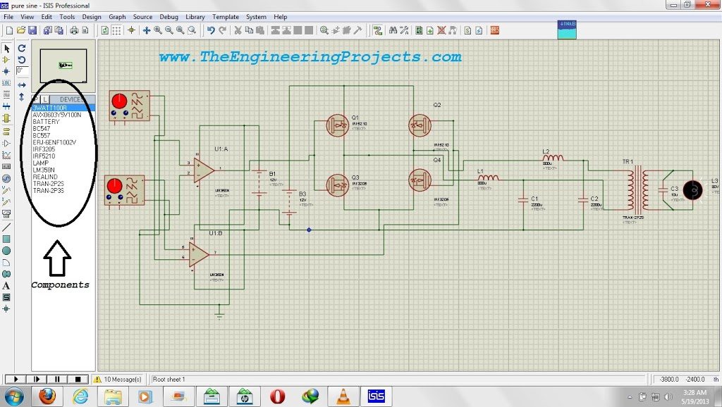
For this lesson, treat that circuit as a source of signals to investigate. The screenshot alone does not establish its distortion, efficiency, device stress, or suitability for a physical inverter. Our immediate question is narrower: what waveform appears at a selected node, and what does the scope actually tell us about it?
If you are learning the controls for the first time, use a low-voltage signal generator and a ground reference before returning to the inverter schematic. A known waveform gives you an expected result. It is easier to understand a scale setting when the source is simple than when both the source and measurement setup are unfamiliar.
Add the Oscilloscope in Proteus
- Open the virtual-instruments mode in the schematic editor.
- Select the oscilloscope instrument.
- Place it near the part of the circuit you want to inspect.
- Connect Channel A to the first measurement node.
- Start the simulation and open the instrument panel.
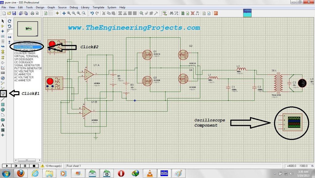
The exact icon arrangement and window controls depend on the Proteus version. Labcenter's oscilloscope-control guide documents the current instrument workflow, including showing a hidden instrument through the running simulation's Debug controls. In older versions, the component's context menu or instrument window controls provide the corresponding operation.
Begin with only the channel you need. Several enabled but unconnected channels create extra lines that can obscure the measurement. Confirm the selected channel is enabled, the simulation is running, and the circuit has an appropriate reference before adjusting more advanced controls.
Set the Vertical Scale
The volts-per-division control determines how much voltage corresponds to one major vertical grid division. If a waveform spans four divisions from its lowest to its highest point and the scale is 2 V/div, its peak-to-peak voltage is 4 × 2 = 8 V.
Choose a range that keeps the complete waveform visible without making it unnecessarily small. If the trace extends beyond the display, increase volts per division. If it occupies only a small fraction of a division, decrease volts per division. Changing the display scale does not change the circuit's actual voltage.
Peak, Peak-to-Peak, and RMS Voltage
Peak-to-peak voltage is the maximum value minus the minimum value. For a symmetrical sine wave centred on zero, peak voltage is half the peak-to-peak value. Its RMS voltage is the peak value divided by the square root of two.
Vpp = Vmax − Vmin; Vpeak = Vpp / 2; Vrms = Vpeak / √2
For an ideal zero-centred 8 V peak-to-peak sine wave, the peak is 4 V and the RMS value is approximately 2.83 V. That RMS shortcut applies to a sine wave under the stated conditions. Do not apply it to a square wave, distorted inverter output, or arbitrary pulse train simply because the scope shows a similar overall height.
A symmetrical square wave switching between +4 V and −4 V also has an 8 V peak-to-peak value, but its RMS value is 4 V. This comparison shows why amplitude alone does not describe the entire waveform.
Screen Position Is Not Circuit DC Offset
The channel-position control moves the trace vertically on the display. It helps separate overlapping traces. It does not inject an offset voltage into the circuit or change the source. To determine a signal's actual DC level, identify its reference and use the measured values rather than judging where the trace happens to sit on the screen.
If you move Channel A upward and Channel B downward for readability, do not then interpret their separation as a voltage difference between the two nodes. Restore comparable references or use a defined differential measurement when the difference matters.
Set the Time Base and Measure Frequency
The time-per-division setting determines the horizontal interval represented by a grid division. To measure a periodic signal, choose two equivalent points on successive cycles, such as rising zero crossings. Their separation is one period, T.
frequency = 1 / period
If one cycle occupies four divisions at 5 ms/div, the period is 4 × 5 ms = 20 ms. Converting to seconds gives 0.020 s, so the frequency is 1 / 0.020 = 50 Hz. Keep the units visible in your calculation; dividing by 20 without converting milliseconds would produce the wrong numerical result.
Choose a time base that shows a few complete cycles for an overview. Then zoom in when examining an edge or a short pulse. If the instrument applies additional horizontal zoom, account for it when interpreting grid spacing, or use its cursor time readout directly.
Measure Pulse Width and Duty Cycle
For a rectangular waveform, measure the interval during which the signal is HIGH and compare it with the full period. A 0.4 ms HIGH interval in a 2 ms period gives a duty cycle of 0.4 / 2 × 100 = 20 percent. The frequency is 1 / 0.002 = 500 Hz.
Changing duty cycle and changing frequency are different operations. A motor-control or servo-control circuit may depend on one or both, so measure them independently. A screenshot showing “some pulses” does not establish that their timing matches the device's requirements.
Stabilize the Trace with Triggering
The trigger establishes a repeatable event from which the display is aligned. For a simple repeating waveform, select the channel carrying that waveform, choose a rising or falling edge, and set a trigger level that the signal actually crosses.
For a pulse varying between 0 V and 5 V, a rising-edge trigger near the middle of that range is a reasonable starting point. If you select a level above the highest signal voltage, that crossing never occurs. Depending on the acquisition mode, the display may appear unstable or may wait for an event that never arrives.
Auto mode is useful while finding a signal. A normal or single-event acquisition is more useful when you want to capture a specific transition and understand why it happened. Changing the trigger changes how the signal is displayed or captured; it does not change the timing of the circuit itself.
Connect Two Channels Across a Load Correctly
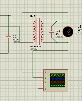
The original screenshot connects Channels A and B to the two sides of the lamp. Each displayed channel represents its node voltage relative to the simulation reference. The voltage across the lamp is their difference, with the sign depending on which side you call positive.
Vload(t) = VA(t) − VB(t)
For example, if one side is at 7 V and the other is at 3 V at the same instant, the load voltage is 4 V. Looking only at the 7 V trace would overstate the voltage across the load. Looking at two traces separately also does not automatically perform their subtraction.
Use the instrument's supported difference operation, or an appropriate inverted-channel summing arrangement, with matching channel scales. Labcenter's control guide explains the available inversion and summing controls. Before interpreting a difference trace, test the setup with two known node voltages so that its polarity and scale are clear.
Comparing Phase and Timing
Two channels can also reveal a time delay between related signals. If corresponding edges differ by 2 ms in a waveform with a 20 ms period, the equivalent phase difference is 360 × 2 / 20 = 36 degrees. State which signal leads and which lags; the magnitude alone does not give the direction of the relationship.
Measure corresponding features, not an arbitrary peak from one waveform and a zero crossing from another. For distorted signals, a single phase figure may not describe all their features. Explain which edge or frequency component the measurement refers to.
Interpret the Original Scope Display
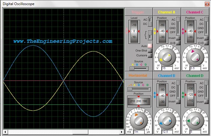
The original running screenshot shows Channels A and B together. Use it to locate the channel controls and understand the comparison workflow. Read each channel's scale and reference before drawing conclusions about amplitude or the voltage across the load.
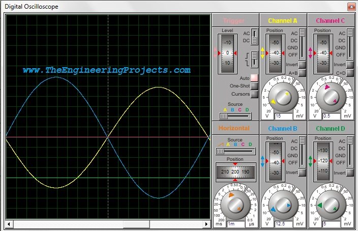
A smooth trace is a useful first observation, but the description “pure sine wave” needs a defined criterion. Harmonics, switching ripple, and distortion can be hidden by the selected scale or limited display resolution. Inspect the waveform at more than one time scale and use suitable spectral or distortion analysis when evaluating an inverter's output quality.
For a periodic signal, total harmonic distortion compares the combined RMS contribution of harmonics with the fundamental RMS component. Conceptually, THD = √(V2² + V3² + ...) / V1, often expressed as a percentage. A time-domain screenshot alone does not provide those individual harmonic values.
Also distinguish startup from steady operation. Inductor current and capacitor voltage can take time to settle after the simulation begins. A large initial transient does not necessarily represent the repeating output, and a clean later waveform does not describe the device stress during startup. State which interval you measured.
AC Coupling and DC Coupling
DC coupling retains both the steady level and changing part of a signal in the measurement path. AC coupling suppresses its DC component, which can make a small ripple easier to view. That does not remove the DC voltage from the actual circuit.
Start with DC coupling when examining logic levels or an unfamiliar node. Use AC coupling deliberately when your question concerns variation around a steady value. Be cautious with very slow signals because the coupling behavior can alter their displayed shape. Keep the channel coupling and trigger coupling settings distinct when the instrument provides both.
Common Measurement Problems
| Observation | Possible explanation | Useful action |
|---|---|---|
| No visible trace | Disabled channel, stopped simulation, or signal outside the display | Enable one channel and choose a wider scale |
| Trace moves continuously | Trigger source or level does not match the signal | Select the connected channel and a valid crossing |
| Waveform appears as a solid band | Too many cycles on screen | Reduce the displayed time interval |
| Waveform is clipped by the screen | Vertical range is too small | Increase volts per division |
| Two equal voltages look different | Different channel scales or positions | Compare numerical values with matching settings |
| A floating load measurement seems wrong | Node voltage mistaken for voltage difference | Measure A minus B with a defined polarity |
Change one setting at a time and note its effect. If you simultaneously alter the source, channel scale, coupling, and trigger, a better picture will not tell you which change solved the problem. Return to a known waveform when the instrument configuration becomes confusing.
Simulation Probes and Physical Oscilloscopes
The virtual instrument makes it easy to inspect circuit nodes, but a physical oscilloscope has input ratings, grounding, bandwidth, and probe-loading limits. Ground connections on a conventional bench oscilloscope can be shared and earth-referenced. Attaching them to arbitrary switching nodes can create a short circuit.
For measurements across floating or high-voltage circuitry, use an appropriately rated measurement arrangement rather than copying virtual probe placement directly onto hardware. Tektronix explains the distinction between single-ended and differential measurements in its probe primer. Keep the instrument's protective earth intact and follow the ratings of the actual probe and oscilloscope.
Video and Suggested Practice
The original video remains below as a visual guide to the older Proteus interface. Use the corrected explanations above when interpreting channel offset, load voltage, and waveform quality.
For practice, connect a simple periodic source to Channel A and measure its period and peak-to-peak voltage. Change only its frequency, predict the new period, and measure again. Then add a second known signal on Channel B and compare their timing with matching display settings.
Finish by moving the channel-position controls without changing either source. Observe that the displayed locations move while the circuit voltages remain the same. This small exercise makes the distinction between screen arrangement and electrical behavior concrete.
Project Review
We have used the Proteus oscilloscope to turn a waveform into measurable quantities instead of treating it as a picture. The essential steps are selecting a reference, choosing useful scales, establishing a trigger, and applying the correct calculation to the signal being measured.
You can apply the same method to the DC power-supply tutorial, motor-drive signals, and serial waveforms. Begin with a specific question, such as ripple amplitude or pulse duration, and configure the instrument to answer that question.
Frequently Asked Questions
Does moving the trace add a DC voltage to my circuit?
No. The channel-position control changes the display position. An actual circuit offset must come from the circuit or its signal source.
Can two channels measure the voltage across a floating load?
In simulation, observe both node voltages and calculate their difference using the appropriate instrument operation. For physical hardware, probe ratings and grounding must also be suitable for that measurement.
Can I calculate RMS from peak voltage for every waveform?
No. Dividing peak voltage by √2 applies to a zero-centred sine wave. Other shapes and signals with a DC component require the appropriate RMS calculation.
Why does the oscilloscope window disappear?
The panel may be hidden while the instrument remains in the schematic. Reopen it using the available instrument or Debug controls during simulation, and check that the simulation is running.
Does a clean-looking sine wave prove an inverter is ready to build?
No. Output distortion, device ratings, protection, thermal behavior, and startup conditions require separate analysis. This tutorial teaches measurement, not a complete hardware qualification process.