Hello friends! Today, we will discuss the operational amplifier, usually called an op-amp. It is one of the most useful building blocks in analog electronics, allowing us to amplify small signals, buffer a sensor, combine voltages and build active filters. The same basic symbol appears in many circuits, but its behavior depends strongly on the components connected around it.
An op-amp responds to the voltage difference between two inputs. By feeding part of its output back to an input, we can obtain a predictable relationship between input and output. This feedback arrangement is the key to understanding practical amplifier circuits.
We will start with the symbol and an ideal model, then introduce the limits of real devices. Along the way, we will calculate common amplifier gains and develop a simple LM358 example. An op-amp does not provide infinite output voltage, unlimited current or noise-free amplification, so these limits must be included in our reasoning.
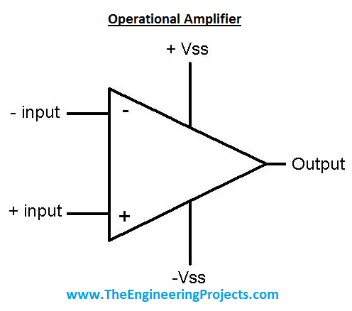
What Does an Operational Amplifier Do?
A conventional voltage-feedback op-amp has a non-inverting input, an inverting input and an output. It also needs power-supply connections, even when a simplified schematic hides them. The three signal terminals are not the complete electrical pinout.
The non-inverting input is marked with a plus sign and the inverting input with a minus sign. These signs describe their effect on the output, not the polarity of the power supply. If the non-inverting voltage rises relative to the inverting voltage, the amplifier tends to drive its output upward.
In a simplified low-frequency model, Vout = AOL(V+ − V−). AOL is open-loop gain, and the parenthesized quantity is the differential input voltage. This relation applies only while the device remains within its operating limits.
For an illustrative open-loop gain of 100,000, a differential input of 10 microvolts requests an output change of 1 V. A 1 millivolt difference would request 100 V, which an amplifier powered from ordinary low-voltage rails cannot provide. The output instead approaches a limiting level and the linear calculation stops applying.
Ideal Assumptions and Real Devices
The ideal model simplifies circuit analysis. It assumes infinite open-loop gain, zero input current, zero output resistance and no offset or noise. These are mathematical assumptions, not specifications of a physical chip. Analog Devices introduces this distinction in its ideal voltage-feedback op-amp tutorial.
| Quantity | Ideal model | Real device |
|---|---|---|
| Open-loop gain | Infinite | Finite and frequency dependent |
| Input current | Zero | Small bias and leakage currents |
| Output resistance | Zero | Finite and affected by feedback and frequency |
| Output range | Unrestricted in an abstract model | Limited by supply, load and output stage |
| Offset and noise | Zero | Present and specified under particular conditions |
| Response speed | Unlimited | Limited by bandwidth, slew rate and settling |
High input impedance means the amplifier draws little current from the signal source. It does not mean current flows freely between the inputs. A high-impedance input is particularly helpful when measuring a source that cannot supply much current without its voltage changing.
The output obtains its energy from the power supply. The input signal controls that energy transfer; it does not magically supply the amplified output power. This is why a correctly drawn feedback network still fails if the amplifier's supply pins are unconnected.
How Negative Feedback Makes Gain Predictable
Negative feedback returns part of the output in a way that opposes the differential input error. In a correctly operating linear circuit, the output moves until the two input voltages are nearly equal. This is often called the virtual-short approximation.
The inputs are not physically shorted together. Almost no current flows between them in the ideal model, and their voltages are only approximately equal when the feedback loop can maintain linear operation. Saturation, excessive frequency or an invalid input range breaks that approximation.
If a circuit needs 3.3 V output and its open-loop gain is 100,000, the simplified model requires a differential input of 3.3/100,000 = 33 microvolts. The small difference explains why treating the input voltages as equal can be useful without claiming that the actual difference is exactly zero.
For feedback factor β, closed-loop gain is AOL/(1 + AOLβ). When loop gain AOLβ is large, the result approaches 1/β. External resistor ratios can therefore determine the useful gain more accurately than relying on the chip's open-loop gain alone.
The Non-Inverting Amplifier
Connect the signal to the non-inverting input. Connect a feedback resistor RF from output to the inverting input, and a resistor RG from the inverting input to the chosen reference, initially ground. For the ideal ground-referenced circuit:
Vout = (1 + RF/RG)Vin.
With RF = 100 kilohms and RG = 10 kilohms, the gain is 11. An input of 0.2 V ideally produces 2.2 V. The output has the same low-frequency polarity as the input, provided the amplifier can support the required input and output voltages.
The resistor divider feeds one-eleventh of the output back to the inverting input. If the output is too low, the non-inverting input is higher and the amplifier raises the output. If it is too high, the feedback voltage exceeds the signal and the amplifier reduces the output.
Resistor tolerance affects the gain ratio. Two separate 1% resistors do not automatically provide a 1% ratio under every combination of errors. For precise amplification, consider the worst-case ratio or use a suitably matched resistor network.
The Inverting Amplifier and Virtual Ground
For an inverting amplifier, connect the non-inverting input to a reference. Feed the signal through an input resistor RIN to the inverting input, and connect RF from output back to that same node. With a ground reference, the ideal relation is Vout = −(RF/RIN)Vin.
With 100 kilohms feedback and 10 kilohms input resistance, gain is −10. An input of +0.2 V requests −2 V output. That example requires an appropriate negative output range; it cannot be reproduced by an ordinary amplifier powered only between ground and +5 V without changing the reference arrangement.
The inverting node stays close to the reference because of feedback. When the reference is ground, we call it a virtual ground. Current entering through RIN flows mainly through RF, not into the amplifier input.
For the 0.2 V example, the input-resistor current is approximately 0.2/10,000 = 20 microamps. The feedback resistor needs a 2 V drop to carry the same current, leading to the −2 V output. This current-based explanation is often easier to follow than memorizing the gain formula.
Voltage Followers and Signal Buffering
A voltage follower connects output directly to the inverting input and applies the signal to the non-inverting input. Its ideal closed-loop gain is one. Although it does not increase voltage amplitude, it can reduce loading on a weak signal source.
Use an amplifier specified as stable at unity gain for this connection. Some devices require a minimum closed-loop gain or a particular feedback network. A direct connection is not a universal instruction for every part described as an operational amplifier.
A buffer also has limited output current and may become unstable with a large capacitive load. Driving a long cable or a large capacitor can require isolation resistance or compensation selected from the device guidance. A gain of one does not remove these practical constraints.
A Practical LM358 Gain-of-Eleven Example
The LM358 contains two amplifiers. In the common eight-pin package, amplifier A uses output pin 1, inverting input pin 2 and non-inverting input pin 3. Pin 4 is the lower supply connection and pin 8 the positive supply. Amplifier B uses pins 5, 6 and 7 for non-inverting input, inverting input and output respectively.
Check the LM358 family datasheet for your exact variant and package. The family includes revised devices with different supply and performance specifications. Its input range includes the negative rail, but it should not be treated as a rail-to-rail-input, rail-to-rail-output amplifier.
- Power the example from a regulated 12 V source, with pin 8 positive and pin 4 at ground.
- Place a 100 nanofarad ceramic bypass capacitor close to the supply pins.
- Connect a 100 kilohm resistor from pin 1 to pin 2.
- Connect a 10 kilohm resistor from pin 2 to ground.
- Apply a slow input between 0.1 V and 0.5 V to pin 3, referenced to the same ground.
- Measure pin 1 with a high-impedance meter or oscilloscope.
The ideal output range is 1.1 V to 5.5 V. That keeps this teaching example comfortably away from the positive supply. Actual readings include resistor error, input offset and other nonidealities. These numbers are calculated expectations, not newly measured bench results.
Do not leave the unused amplifier's inputs floating. Configure it in a stable defined arrangement, such as a follower with its non-inverting input tied to a valid reference voltage within the common-mode range. Avoid connecting its output directly to a supply rail.
Before applying a varying signal, check the DC supply and input voltages. A feedback resistor connected to the wrong input can create positive feedback, causing the output to stick near a limit instead of following the intended gain.
Input Range and Output Swing Are Different Limits
The common-mode input voltage is the average of the two input voltages. An amplifier can have a tiny differential input and still fail if both inputs sit outside the permitted common-mode range. Check that range at the actual supply and temperature conditions.
Output swing is another specification. An amplifier powered from 0 V and 5 V cannot normally produce −2 V or +10 V. Even within those rails, the usable output range depends on the device and load. Rail-to-rail terminology still comes with conditions and finite headroom.
On a single supply, an AC signal may need a mid-supply reference. If an inverting stage is referenced to VREF, its ideal equation becomes Vout = VREF − (RF/RIN)(Vin − VREF). The reference must itself remain sufficiently stable under the circuit's loading.
Bandwidth, Slew Rate and Settling
Open-loop gain decreases as frequency rises. For a simple dominant-pole voltage-feedback amplifier, closed-loop bandwidth is approximately gain-bandwidth product divided by noise gain. This is a useful estimate, not a universal formula for every amplifier architecture.
For a hypothetical 1 MHz gain-bandwidth product and non-inverting gain of 11, the approximate small-signal bandwidth is 91 kHz. Operation near that bandwidth already involves significant amplitude and phase error. Choose margin rather than treating the bandwidth limit as a perfectly flat operating region.
Slew rate limits how quickly the output voltage can change. A sine wave with peak amplitude Vpk requires a maximum slope of 2πfVpk. At 10 kHz and 1 V peak, that is about 0.0628 V per microsecond.
If the amplifier cannot provide the required slope, the waveform distorts even when a small-signal bandwidth calculation seems acceptable. Settling time adds another consideration: after a step, the output must approach the requested value closely enough for the intended measurement.
Offset, Bias Current and Noise
Input offset voltage represents a small input-referred error. In a gain-of-eleven non-inverting circuit, an illustrative 2 mV offset can contribute approximately 22 mV at the output. Use the chosen part's limits and drift specifications when developing an error budget.
Input bias current flowing through source resistance also produces a voltage error. A hypothetical 50 nA through 100 kilohms gives 5 mV. This explains why choosing extremely large resistors can make a circuit sensitive to effects ignored by the ideal model.
Real amplifiers and resistors generate noise. Amplifying a weak signal also amplifies noise already present within the circuit's passband, while the amplifier contributes its own noise. Increasing gain does not automatically improve signal-to-noise ratio.
Filtering can reject frequencies outside the wanted band. For a first-order RC low-pass network, fc = 1/(2πRC). A 10 kilohm resistor and 100 nanofarad capacitor give a corner near 159 Hz. That network also attenuates and phase-shifts wanted signals near its corner, so its value must follow the application's bandwidth requirement.
Other Useful Op-Amp Applications
A summing amplifier combines currents from several input resistors into a feedback node. With equal input resistors, the output can represent a scaled negative sum of the inputs. This is useful for combining or offsetting analog signals.
A difference amplifier subtracts two signals with a resistor network. Its rejection of a shared common-mode voltage depends strongly on resistor matching as well as amplifier performance. For demanding small differential measurements, an instrumentation amplifier may provide a more suitable architecture.
An integrator uses a capacitor in the feedback path. In the ideal circuit, output changes according to the accumulated input over time. A practical integrator usually needs a DC feedback path or reset arrangement because offset and bias current can otherwise drive the output into saturation.
Op-amps also appear in active filters, photodiode interfaces and converter signal conditioning. They do not automatically form a complete ADC or DAC simply by being present. Each application adds its own requirements for gain, stability, range and error.
Why an Op-Amp Is Not Always a Good Comparator
A comparator decides which of two voltages is larger and produces an output intended for that decision. An op-amp is generally optimized for linear operation with feedback. Using it open-loop can produce slow recovery from saturation, unsuitable output levels or problems with differential-input limits.
Texas Instruments discusses these limitations in its guidance on using op-amps as comparators. For a new threshold-detection circuit, select a comparator whose input range, output type and timing match the application rather than assuming an amplifier is automatically faster.
Hysteresis can prevent a threshold detector from switching repeatedly when a noisy signal sits near the decision level. That is a deliberately designed positive-feedback function, distinct from the negative feedback used for linear amplification.
Troubleshooting and Design Review
| Observation | Check |
|---|---|
| Output stuck near a rail | Feedback polarity, input range and requested output voltage |
| Gain differs from calculation | Resistor ratio, loading and frequency |
| Output oscillates | Unity-gain stability, capacitive load, layout and bypassing |
| Small DC error appears | Offset voltage, bias current and reference accuracy |
| Large signals distort | Output swing, current limit and slew rate |
| Noise increases with gain | Input noise, resistor values, bandwidth and grounding |
Start with a simple DC test before adding a complicated sensor or waveform. Measure both supply pins, both inputs and the output relative to the intended reference. Then compare the measurements with the feedback equation and the device limits. This sequence often reveals a wiring or range problem quickly.
Frequently Asked Questions
Does an op-amp have only three pins?
No. The basic symbol has three signal terminals, but the device also needs supply connections and may contain multiple amplifiers or additional functions.
Are the two input voltages always equal?
No. They are approximately equal only when suitable negative feedback maintains linear operation within the amplifier's limits.
Can an op-amp remove all noise from a signal?
No. It adds its own noise and amplifies in-band noise already present. A properly designed filter can reduce unwanted frequency components, but cannot make every signal noise-free.
Is the inverting input normally connected to ground?
It depends on the circuit. In common amplifier configurations, it participates in the feedback network. A virtual ground is a controlled voltage condition, not a physical ground connection.
Can the LM358 drive a motor directly?
It is a signal amplifier, not a motor power stage. Use an appropriate driver and protection circuit for the motor's current and inductive behavior.
What should I calculate first?
Start with the required input and output ranges, supply voltage, gain and signal bandwidth. Then choose a device and resistor network that meet those requirements with suitable margin.