Hello friends! Today we will detect coloured objects in an image using MATLAB, draw their bounding boxes and calculate their centre coordinates. We will keep the original demonstration with red, green and blue shapes, then explain what changes when the input is a real photograph.
In our circle-detection tutorial, we selected objects by geometry. Here, we first select pixels by colour and then group neighbouring selected pixels into regions. A green triangle and a green circle can both be detected because colour, rather than shape, is the initial rule.
We will use a reusable script with explicit colour thresholds and a minimum object area. The settings are starting values for a demonstration image, not universal definitions of red, green and blue under every camera and lighting condition.
Understand the Colour-Detection Workflow
The process has three distinct stages. Segmentation decides which pixels match the chosen colour. Connected-component analysis groups those pixels into regions. Measurement calculates a bounding box, centroid and area for each retained region.
A region is not automatically a complete physical object. Two touching green objects can become one region, while a shadow can split one object into several regions. We must keep that distinction in mind when reporting an object count.
| Stage | Input | Output |
|---|---|---|
| Colour conversion | RGB image | Channels suitable for threshold selection |
| Thresholding | Channel values and chosen limits | Logical foreground mask |
| Small-region removal | Mask and minimum area | Cleaned mask |
| Region measurement | Connected foreground regions | Area, centroid and bounding box |
| Display and review | Measurements and original image | Annotated result |
Prepare the Test Image and MATLAB
You need MATLAB with Image Processing Toolbox for the complete example. Save the image in your working folder or provide its full path. If you need help creating a script, see How to Create an m File in MATLAB.
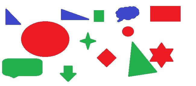
The original image contains deliberately simple shapes on a light background. It is a good first example because the intended colour groups are easy to identify. Start with this kind of controlled input before attempting outdoor photographs or reflective objects.
Use the actual image file, not a screenshot containing browser controls or annotations. Text and coloured borders in a screenshot can become additional detected regions. Resizing the image also changes the number of pixels occupied by each shape.
The updated script accepts an RGB image or an indexed image that can be converted through its palette. It rejects ordinary grayscale input because a single intensity channel does not contain the original colour information.
Why Use HSV for This Example?
RGB stores red, green and blue channel intensities. HSV expresses the same image in terms of hue, saturation and value. This often makes a simple colour-selection rule easier to describe.
Hue represents position around a colour wheel. Saturation indicates how strongly coloured a pixel is compared with a neutral shade. Value corresponds to the largest RGB component in the conversion used here.
The rgb2hsv documentation describes MATLAB's normalized ranges. For floating-point RGB input, use values in the expected zero-to-one range. Converting uint8 data with im2double performs the required intensity scaling; simply calling double leaves values on their original numerical scale.
Hue is circular. Red appears near both zero and one, so a red threshold generally needs two intervals joined with OR. Green and blue can be represented by single intervals for this simple experiment.
| Colour | Example normalized hue rule | Additional restrictions |
|---|---|---|
| Red | H at most 0.05 or H at least 0.95 | S at least 0.35 and V at least 0.20 |
| Green | H from 0.25 to 0.45 | S at least 0.35 and V at least 0.20 |
| Blue | H from 0.55 to 0.75 | S at least 0.35 and V at least 0.20 |
The saturation restriction helps reject white and gray backgrounds, where hue is not a useful indicator of a strong colour. The value restriction rejects very dark pixels whose apparent hue can be unstable. Adjust both based on your actual target.
Complete MATLAB Colour-Detection Script
Set targetColor to red, green or blue. Start with the same minimum area of 300 pixels used in the original tutorial, then change it if the image scale or intended object size requires a different value.
imagePath = 'TEP1.jpg';
targetColor = 'green';
minimumArea = 300;
minimumSaturation = 0.35;
minimumValue = 0.20;

[A, map] = imread(imagePath);
if ~isempty(map)
    rgbImage = ind2rgb(A, map);
elseif ndims(A) == 3 && size(A,3) == 3
    rgbImage = im2double(A);
else
    error('Select an RGB or indexed colour image.');
end

hsvImage = rgb2hsv(rgbImage);
H = hsvImage(:,:,1);
S = hsvImage(:,:,2);
V = hsvImage(:,:,3);

switch lower(targetColor)
    case 'red'
        hueMask = H <= 0.05 | H >= 0.95;
    case 'green'
        hueMask = H >= 0.25 & H <= 0.45;
    case 'blue'
        hueMask = H >= 0.55 & H <= 0.75;
    otherwise
        error('targetColor must be red, green or blue.');
end

rawMask = hueMask & S >= minimumSaturation & V >= minimumValue;
cleanMask = bwareaopen(rawMask, minimumArea, 8);
components = bwconncomp(cleanMask, 8);
stats = regionprops(components, 'Area', 'Centroid', 'BoundingBox');

figure;
subplot(1,2,1);
imshow(cleanMask);
title([targetColor ' mask']);
subplot(1,2,2);
imshow(rgbImage);
hold on;
for k = 1:numel(stats)
    box = stats(k).BoundingBox;
    centre = stats(k).Centroid;
    rectangle('Position', box, 'EdgeColor', 'y', 'LineWidth', 2);
    plot(centre(1), centre(2), 'm+');
    text(centre(1)+5, centre(2), ...
        sprintf('%d: x=%.1f y=%.1f', k, centre(1), centre(2)), ...
        'Color', 'black', 'BackgroundColor', 'white');
end
hold off;
title(sprintf('%d %s regions', numel(stats), targetColor));

measurements = regionprops('table', components, ...
    'Area', 'Centroid', 'BoundingBox');
disp(measurements);
This script measures all retained regions without assuming at least one exists. An empty result can be valid when the chosen colour is absent. It can also indicate that thresholds or the minimum-area setting need adjustment.
The original file was called TEP.jpg in the code, while the image resource used another filename. Use the name of the file you actually saved. A file-not-found error is unrelated to colour thresholds.
Detect Green, Red and Blue Shapes
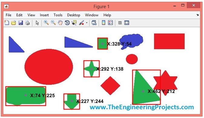
Run the script with targetColor set to green and inspect the mask beside the annotated source. Foreground pixels should cover the green shapes, while the background and differently coloured shapes remain excluded.
The retained green result demonstrates the original method's intended output. The updated HSV workflow may produce slightly different boundaries and annotations. These historical screenshots should not be interpreted as fresh output from the revised code.
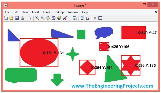
Change targetColor to red and run the script again. The OR between the low and high hue intervals is important. Requiring both conditions simultaneously would select nothing because one hue value cannot be near both ends at the same time.
Finally select blue. Keep the source image and all other parameters fixed for this initial comparison, so the effect of changing the colour rule is clear.
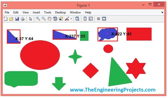
To detect all three groups in one project, run the masks separately and attach the colour name to each measurement. If you later widen ranges until they overlap, define a policy for ambiguous pixels rather than silently counting the same region twice.
Understand the Original RGB-Subtraction Method
The earlier tutorial subtracted a grayscale image from one RGB channel. For example, subtracting grayscale from the green channel emphasizes pixels where green is strong relative to the grayscale mixture.
That is a useful colour-excess demonstration, but changing the selected channel does not make the threshold equally sensitive to every colour. Grayscale conversion weights the channels differently, and integer subtraction can clip negative differences.
The old im2bw call is also no longer the recommended general conversion workflow. MathWorks identifies its replacement options in the im2bw reference. For the explicit logical comparisons used in our HSV script, there is no need to convert the already logical mask again.
When comparing the old and new approaches, show both masks on the same input. Neither a pleasant overlay nor a larger region count proves that one method is better. Evaluate whether the selected pixels match the actual objects of interest.
Remove Noise Without Removing the Target
The bwareaopen function removes connected foreground regions smaller than the specified pixel count. The value 300 is an area threshold, not a brightness threshold or a distance in millimetres.
If a legitimate object contains only 180 selected pixels, a threshold of 300 removes it completely. Lower the threshold only after inspecting whether small unwanted regions will then survive as well.
Image scaling affects area quadratically. Resizing both dimensions by one half reduces an object's pixel area to about one quarter. A 300-pixel threshold at full resolution corresponds roughly to 75 pixels after that uniform reduction.
Morphological opening, closing or hole filling can be useful, but each operation changes geometry. Closing can merge nearby objects; filling can remove meaningful holes. Do not automatically add every cleanup function just because the mask looks smoother afterward.
Choose the Connected-Component Rule
The script uses eight-connectivity: diagonally touching foreground pixels can belong to the same component. Four-connectivity uses only edge-sharing neighbours. That choice can change the number of measured regions along thin diagonal connections.
Use the same connectivity when removing small regions and when constructing components. Otherwise, cleanup and measurement can disagree about what constitutes an object.
If two green objects touch, colour alone may not separate them. You may need shape information, an expected size model, a separating boundary or an additional segmentation method. Raising the minimum area cannot split a merged region.
Likewise, a patterned object may contain disconnected patches of the same colour. A component count measures those patches unless your algorithm includes a justified rule for associating them with one object.
Read the Centroid, Bounding Box and Area
The regionprops reference defines these measurements. A centroid is the mean position of the selected pixels in a region. It is not necessarily the centre of the bounding rectangle or the physical centre of a three-dimensional object.
For N foreground pixels, the binary centroid follows xc = sum(xi)/N and yc = sum(yi)/N. A missing patch caused by glare shifts that mean, even if the physical object has not moved.
The bounding box contains a position and width/height in image coordinates. Its purpose is to enclose the selected region. Do not confuse its first two values with the centroid.
MATLAB uses row-column array indexing, but centroid coordinates are x,y. In a conventional image display, x increases rightward and y increases downward. Preserve floating-point centroids for measurement and round only when an operation specifically needs an integer pixel index.
Area counts selected pixels. If a calibrated planar image has scale s millimetres per pixel, the approximate area is N x s2 square millimetres. This assumes the scale is valid across that region and does not correct perspective or an incomplete mask.
Tune Thresholds with the Colour Thresholder App
For an unfamiliar photograph, manually guessing hue bounds can be slow. The Colour Thresholder workflow lets you inspect colour distributions and interactively adjust the selected region.
Load a representative image, compare available colour spaces, select limits and inspect both foreground and background errors. Export the resulting mask function when the selected rule is useful, then keep its parameters with the project.
Try examples with shadows and bright reflections before finalizing thresholds. A rule selected from one perfectly lit object can exclude the same object when it rotates or moves closer to a lamp.
Keep a note of the camera exposure, white balance and lighting arrangement. Automatic camera adjustments can shift channel values between frames even when the object itself is unchanged. Stable illumination is often more valuable than increasingly complicated threshold expressions.
Recognize the Limits of Colour Alone
HSV is not immune to illumination changes. A coloured light changes the image's colour balance, while a bright reflection can make a saturated surface appear nearly white. A dark shadow may fail the minimum-value requirement.
A red object against a red background cannot be reliably separated by a rule that only asks whether each pixel is red. Add location, shape, texture or depth information when the scene requires it.
For a fixed inspection station, control the background, camera position and lighting. For a mobile camera, plan a wider range of test conditions and expect that fixed thresholds may need replacement by a more capable method.
Do not interpret RGB or HSV values as calibrated physical colour measurements without the appropriate imaging and calibration procedure. This tutorial is about segmenting image regions, not certifying a material's colour specification.
Evaluate the Mask and the Object Count
A region of interest can make this evaluation easier. Suppose a conveyor occupies the central part of a frame, while a red indicator lamp sits above it. Restrict processing to the conveyor when the lamp is outside the task. Record that restriction explicitly; otherwise a change in camera position may move valid objects outside the accepted region without changing any colour threshold.
If you crop the image before processing, measurements initially belong to the crop. For a crop whose top-left pixel is at original column x0 and row y0, recover full-image coordinates with x = xcrop + x0 - 1 and y = ycrop + y0 - 1. The subtraction accounts for MATLAB's one-based pixel coordinates. Alternatively, retain the full image and combine the colour mask with a logical region-of-interest mask of the same dimensions.
Choose test images that answer different questions. Include an empty scene to reveal background false detections, a small distant object to challenge the area threshold, touching objects to expose merging, and a partly shaded object to expose fragmentation. Include at least one example that should be rejected even though part of it has the target colour.
Keep threshold selection separate from the final assessment. When a new failure appears, record the reason before adjusting a parameter. Lowering saturation may recover a faded target but admit a neutral background; reducing the area cutoff may recover a small object but admit noise. Compare both gains and losses across the saved examples rather than judging the change from the latest image alone.
Create reference masks for a small set of representative images. Compare selected and missed pixels, then separately compare detected regions with the intended objects. A good pixel score can still hide a merged pair of objects.
Intersection over union is a useful mask measure: the number of pixels selected by both prediction and reference divided by the number selected by either. If the intersection contains 800 pixels and the union contains 1000, IoU is 0.80.
For object detection, record false detections and missed objects. Define how close a centroid and region size must be to count as a match. Keep a separate evaluation set so threshold tuning does not simply memorize the examples used to choose it.
Save the source image, target colour, thresholds, minimum area and measurement table together. This makes a reported result traceable and lets you distinguish a changed image from a changed algorithm.
Common Problems and Practical Review
| Problem | Likely reason | Next step |
|---|---|---|
| White background detected as red | Hue used without saturation restriction | Inspect saturation and reject neutral pixels |
| Small intended objects disappear | Minimum area exceeds their selected area | Recalculate the threshold for image scale |
| One object becomes several regions | Shadow, reflection or disconnected colour patches | Inspect the raw mask before cleanup |
| Two objects become one | Their selected pixels touch | Add a justified separation method |
| Coordinates are transposed | Row-column and x,y were confused | Check the measurement convention |
| Colour rules fail after changing camera | Different image response or lighting | Recalibrate on representative inputs |
Our MATLAB image-processing projects provide further exercises. For this tutorial, concentrate on understanding the mask first: every reported bounding box and centroid depends on which pixels the mask accepted.
Frequently Asked Questions
Does the script recognize the shape of an object?
No. It initially selects colour. Add geometric measurements if you need to distinguish a circle from a triangle of the same colour.
Why does red need two hue ranges?
The hue scale wraps around, placing red near both ends of the normalized interval.
Can I use the same thresholds for every photograph?
Not reliably. Camera settings, lighting, background and target appearance affect the useful limits.
Is the centroid always inside the detected object?
Not necessarily. For a concave region or a ring, its mean position can fall in a gap or excluded area.
Can this be extended to video?
Yes. Apply the processing to each frame, then add timing, stable identifiers and tracking if object identity across frames matters.