Hello friends! Today, we are going to discuss power factor measurement using a microcontroller in Proteus. We will use the ATmega8 project to understand how the timing difference between voltage and current can be converted into a phase angle, and then into a power factor reading on an LCD.
I will start with the electrical meaning of power factor, because a correct calculation is useful only when we understand what it measures. After that, we will examine the zero-crossing stages, choose a timer resolution, work through numerical examples and discuss the changes needed for reliable firmware.
The circuit is an educational simulation using separate signals to represent voltage and current. Its timing method is appropriate for sinusoidal waveforms. When a load draws distorted current, we need an additional measurement approach to obtain true power factor, which we will also explain.
What Does Power Factor Tell Us?
Power factor describes the relationship between real power and apparent power in an AC circuit. Real power, measured in watts, is the average rate of energy transfer. Apparent power, measured in volt-amperes, is the product of RMS voltage and RMS current. Their ratio is dimensionless:
PF = P / S = P / (Vrms × Irms)
For example, suppose a load takes 230 V RMS and 2 A RMS, while its measured real power is 230 W. Its apparent power is 460 VA, so its power factor is 0.5. This calculation does not tell us how efficiently the load converts electrical input into mechanical motion, heat or another useful output.
A power factor of 0.5 does not mean 50% efficiency. Efficiency compares useful output power with input real power. Power factor compares input real power with input apparent power. Confusing these quantities leads to incorrect explanations of both energy consumption and equipment performance.
A lower power factor can require more current to deliver the same real power at a fixed voltage. That additional current can increase resistive losses in cables and equipment. However, we cannot simply call the remaining percentage of apparent power wasted energy.
Resistive, inductive and capacitive loads
For an ideal resistor, sinusoidal current follows sinusoidal voltage without a phase displacement. An inductive load can make current lag voltage, while a capacitive load can make current lead voltage. Real equipment usually combines resistance with reactive behavior, so its phase angle lies between the ideal limiting cases.
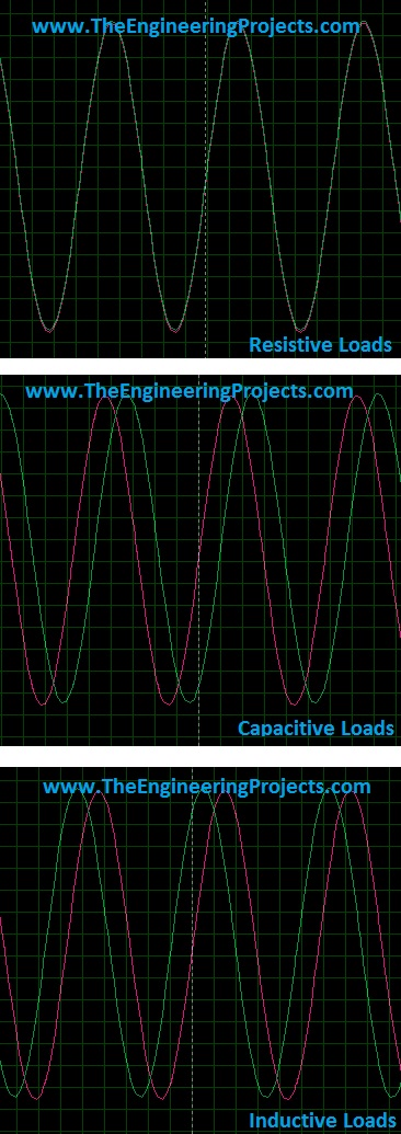
The original illustration compares these three relationships. Use the waveform labels and the direction of time when identifying which signal leads. A curve that reaches the same point in its cycle earlier is the leading signal. Comparing unrelated peaks or opposite zero crossings can produce a misleading angle.
Ideal inductors and capacitors alternately store energy and return it to the source. Their reactive behavior is different from irreversible heating in a resistor. Practical components also have resistance and other losses, but those losses should be discussed separately from the phase relationship.
Displacement Power Factor and True Power Factor
When voltage and current are sinusoids of the same frequency, the familiar expression is PF = cos(φ), where φ is their phase difference. The zero-crossing project estimates this phase relationship. In this setting, a zero-degree displacement gives a power factor of 1, while a 60-degree displacement gives 0.5.
Many electronic loads draw pulses of current rather than a clean sine wave. A single zero-crossing time does not describe the shape of those pulses. Consequently, a phase measurement can look satisfactory even while RMS current is much greater than a sinusoidal model would suggest.
We should therefore label a zero-crossing result as displacement power factor unless the waveform conditions justify calling it true power factor. Analog Devices explains the distinction in its power factor and cos(φ) discussion.
| Measurement | Required information | What this project provides |
|---|---|---|
| Phase displacement | Corresponding voltage and current edges | A timing-based estimate |
| Displacement power factor | Cosine of the fundamental phase angle | An estimate for clean sinusoidal inputs |
| True power factor | Average real power and both RMS quantities | Not established by zero crossings alone |
| Efficiency | Useful output power and input real power | Not measured by this circuit |
Understanding the Proteus Circuit
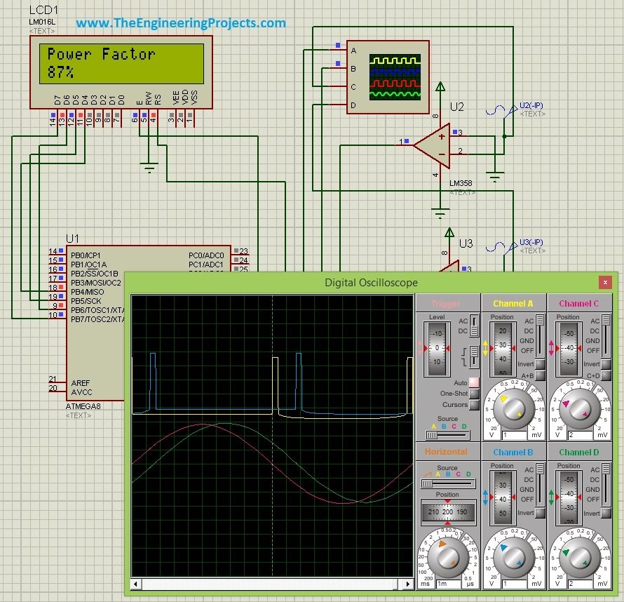
The original project contains an ATmega8, LM358 stages, two AC signal sources, a 16×2 LCD and an oscilloscope. One signal represents the conditioned voltage channel; the other represents the conditioned current channel. We change their relative phase to investigate different operating conditions.
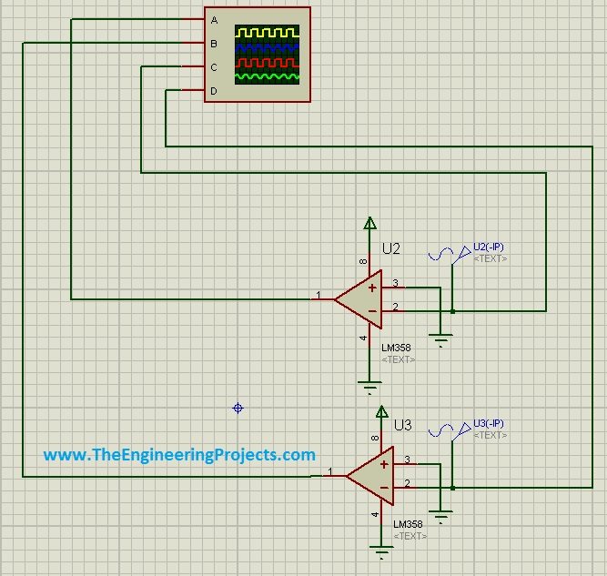
These sources make the timing exercise convenient because we can set frequency and phase without building a complete power-measurement front end. They do not simulate every property of a voltage transformer, current transformer, protection network or physical load. Keep that distinction in mind when interpreting the result.
The ATmega8 receives logic transitions from the conditioning stages. Its timer measures elapsed counts, and the program converts those counts into a phase estimate. The LCD is the final display; it does not improve the accuracy of the acquisition stage.
What a zero-crossing detector actually produces
A comparator changes output state when the relationship between its two inputs changes. With an appropriate reference, its transitions identify crossings of that reference level. Depending on input polarity, a rising output edge may correspond to either the positive-going or negative-going crossing of the original waveform.
This operation is not a conversion of an AC supply into regulated DC. We are producing a logic-compatible representation of waveform polarity. The useful timing information is in the transitions, not in the fact that an output happens to remain high for part of a cycle.
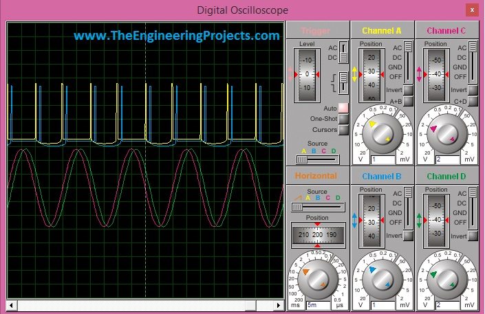
The original oscilloscope capture shows the two analog waveforms and the detector outputs. Inspect the transitions against the analog crossings before trusting the LCD. A narrow spike, extra transition or unequal channel delay can give the software the wrong event to measure.
Limits of the LM358 demonstration
The LM358 is an operational amplifier, and its behavior as an open-loop detector should not be assumed identical to a dedicated comparator. Input range, output swing and recovery behavior depend on the particular device and operating conditions. Consult the applicable Texas Instruments LM358 documentation before designing a physical front end.
In particular, a single-supply circuit cannot accept an arbitrary bipolar signal simply because its peak magnitude is below 5 V. Negative input excursions, logic thresholds and output voltage limits all matter. A practical low-voltage detector needs suitable signal conditioning, a defined reference and compatible input/output ranges.
For this tutorial, work with isolated low-voltage signals. The schematic is not a complete mains-connected instrument. Isolation, transient protection and safe physical construction require their own design; adding a transformer symbol in Proteus does not establish those properties.
Calculating Phase Angle from Time Difference
Let T be the period of the voltage waveform. Let Δt be the signed time difference between corresponding current and voltage crossings. If we define Δt as current time minus voltage time, positive values describe lagging current and negative values describe leading current within the selected cycle.
φ in degrees = 360 × Δt / T
φ in radians = 2π × Δt / T
Displacement PF = cos(2π × Δt / T)
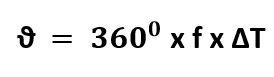
Since T = 1/f, the same calculation can be written using frequency. Measuring the actual period is often more useful than assuming the signal remains exactly at 50 Hz or 60 Hz. It also lets the program reject missing, implausible or unstable input periods.
| Frequency | Period | Time displacement | Angle magnitude | Cosine |
|---|---|---|---|---|
| 50 Hz | 20 ms | 0 ms | 0° | 1.000 |
| 50 Hz | 20 ms | 1.6667 ms | 30° | 0.866 |
| 50 Hz | 20 ms | 3.3333 ms | 60° | 0.500 |
| 60 Hz | 16.6667 ms | 1.3889 ms | 30° | 0.866 |
Notice that the same phase angle has a different time displacement at a different frequency. A program that always multiplies by 50 will be wrong when the signal is actually 60 Hz. Also, ordinary C cosine functions expect radians, so a degree value must be converted before calling them.
Choosing the ATmega8 Timer Configuration
The ATmega8 includes a 16-bit Timer/Counter1 with capture facilities. Its clock selection and prescaler determine the duration represented by one count. The device's pin functions and timer operation are documented in the ATmega8 datasheet.
For an illustrative configuration using an 8 MHz timer source and a divide-by-eight prescaler, the counter advances at 1 MHz. Each count then represents one microsecond. A 20 ms signal period occupies approximately 20,000 counts, and a full 16-bit wrap takes 65.536 ms.
That calculation is a configuration example, not a claim about the clock used in every archived project file. Check the actual oscillator settings, simulation clock and timer register values together. Dividing a count by one million is correct only when the counter really advances one million times per second.
The historical program observes PC4 and PC3. Those general-purpose input bits do not become hardware capture inputs just because Timer1 is running. A redesigned acquisition system can use suitable interrupt or capture pins, but that requires matching schematic changes and a deliberate choice of edge polarity.
A reliable acquisition sequence
- Confirm that both channels have valid logic levels and the expected waveform frequency.
- Record a selected voltage edge, such as the transition associated with a positive-going crossing.
- Record the corresponding current edge using the same analog crossing direction.
- Record the next voltage edge to measure a complete period.
- Handle counter wrap, reject stale measurements and calculate the signed displacement.
- Update the displayed result only after the complete measurement passes validation.
Use a timeout for every stage that depends on an external event. If the current signal disappears, the firmware should report an invalid measurement instead of waiting forever or displaying the last number as though it were new.
With an 8-bit processor, a multi-byte timestamp can change while the main program is reading it. Use the compiler and device's recommended atomic-access approach when sharing values with an interrupt routine. Keep acquisition routines short; LCD formatting and floating-point calculations belong outside time-critical interrupt code.
A Clear Calculation Function
The following standard C example handles the arithmetic after valid timestamps have already been collected. It is not a replacement for the complete project firmware: the acquisition, LCD driver, clock setup and error reporting still need to be implemented for the chosen compiler and circuit.
#include <stdint.h>
#include <math.h>

int calculate_displacement_pf(uint16_t period_ticks,
                              int32_t current_minus_voltage,
                              float *angle_degrees,
                              float *power_factor)
{
    int32_t period;
    int32_t delta;
    float radians;

    if (period_ticks == 0 || angle_degrees == 0 || power_factor == 0)
        return 0;

    period = (int32_t)period_ticks;
    delta = current_minus_voltage % period;
    if (delta > period / 2) delta -= period;
    if (delta < -period / 2) delta += period;

    radians = 6.28318530718f * (float)delta / (float)period;
    *angle_degrees = 360.0f * (float)delta / (float)period;
    *power_factor = cosf(radians);
    return 1;
}
Because both inputs use the same timer units, their ratio does not require a separate conversion to seconds. The signed displacement is normalized into the nearest half-cycle interval. This normalization is useful for phase arithmetic, but it cannot detect a disconnected sensor or prove that two captured edges belong to a valid measurement.
Do not take an absolute value merely to make every result positive. Depending on the measurement convention, a negative real-power relationship can carry useful information about power direction. For the simple consuming loads discussed here, display the cosine together with a separate leading or lagging indication.
Likewise, avoid always rounding upward. A calculated value of 0.866 can be displayed as 0.87 through ordinary rounding. Calling it 87% is a presentation choice, but the screen should not label that percentage as efficiency.
Running the Original Proteus Project
The original complete simulation was offered separately through the power factor measurement project page. Refer to that page for its current availability and supplied files. The explanation here preserves the original project context without assuming an old price or package remains unchanged.
- Open the project and identify the voltage and current signal channels.
- Check the ATmega8 program-file path and clock setting against the firmware build.
- Set both sources to the same frequency, initially with zero phase displacement.
- Observe the analog and detector signals on the oscilloscope.
- Introduce a known phase difference and compare the display with a manual calculation.
- Repeat with leading and lagging current rather than checking only one direction.
The original capture displays approximately 0.87 for a 30-degree relationship. That is consistent with cos(30°) ≈ 0.866. It demonstrates the intended calculation, but a screenshot alone does not establish calibration, harmonic performance or physical-hardware accuracy.
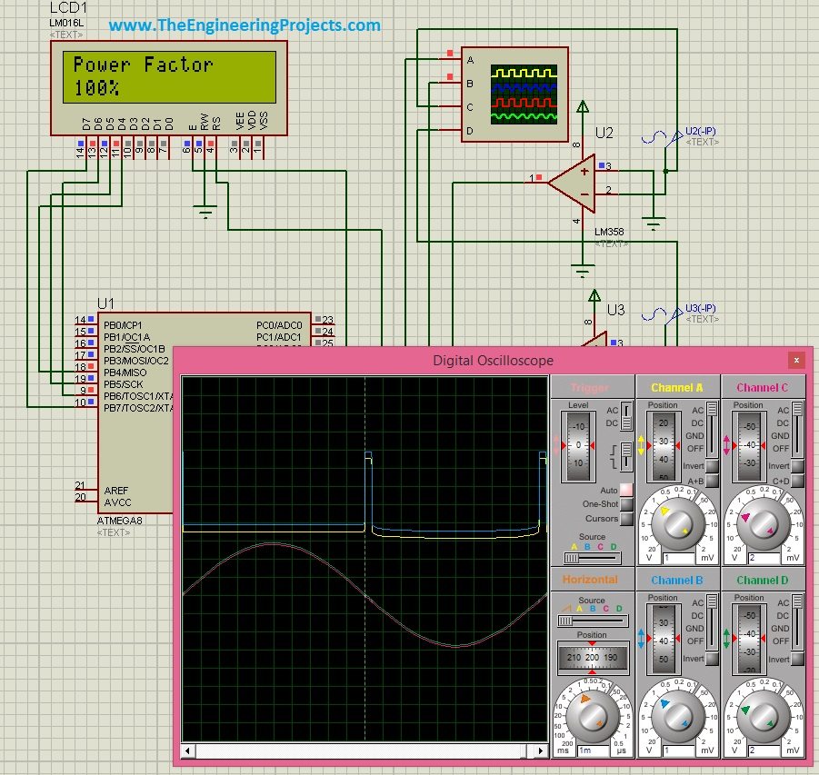
When corresponding crossings coincide, the intended result is approximately 1.00. If it is not, inspect channel polarity, threshold offsets and acquisition delay before changing the formula. An incorrect edge pair can produce an apparently stable but incorrect reading.
Accuracy, Calibration and Error Handling
Timing error becomes phase error. At 50 Hz, a 50 microsecond timing mismatch represents 360 × 50 µs / 20 ms = 0.9°. The effect on the final cosine depends on the operating angle, so the same timing error does not produce the same power-factor error everywhere.
Near 60 degrees, a small-angle estimate gives a power-factor change of approximately sin(60°) × 0.9π/180 ≈ 0.014. This illustrates why a display with two decimal places does not automatically provide two-decimal accuracy.
Feed both channels with the same suitable low-voltage test signal to examine their relative timing offset. Then repeat at different amplitudes and frequencies. A fixed calibration correction may remove a fixed offset, but it cannot compensate every amplitude-dependent threshold effect or transformer phase error.
Noise near a crossing can create multiple transitions. Hysteresis and filtering can help, but they also influence timing. Apply comparable conditioning to both channels and characterize the remaining mismatch instead of assuming that every added filter improves accuracy.
| Symptom | Likely issue | Useful check |
|---|---|---|
| Reading always equals one | Both tests detect an existing high level | Capture transitions rather than static states |
| Reading changes with display updates | Acquisition is delayed by blocking work | Separate timing from LCD formatting |
| Correct at 50 Hz but wrong at 60 Hz | Fixed-frequency conversion | Measure the period |
| Occasional large jumps | Extra edges, overflow or torn timestamps | Inspect validity checks and atomic reads |
| Number remains after input removal | No freshness timeout | Display an invalid or missing-signal state |
How Would We Measure True Power Factor?
For distorted waveforms, acquire calibrated voltage and current samples with an appropriate sampling rate and controlled timing relationship. Over a suitable observation interval, calculate average instantaneous power and both RMS values.
P = Σ(v[n] × i[n]) / N
Vrms = √(Σv[n]² / N), Irms = √(Σi[n]² / N)
Then calculate PF = P / (Vrms × Irms), provided the denominator is valid. Sensor offsets, sampling skew, bandwidth and anti-alias filtering now become part of the design. This is a different acquisition problem from observing only two logic transitions per cycle.
Project Review
This project is useful for learning phase relationships, comparator timing and timer-based measurement. Its strongest teaching feature is that you can change the simulated phase and immediately connect that change with a numerical calculation. Its main limitation is that zero-crossing timing does not fully characterize arbitrary load waveforms.
A sensible extension is to add measured frequency, leading or lagging status and explicit invalid-input messages. Complete those functions before adding more display precision. A trustworthy instrument should explain when its measurement is unavailable as clearly as it displays a valid result.
Frequently Asked Questions
Does a power factor of 0.5 mean half the energy is wasted?
No. It means real power is half the apparent power under the stated measurement conditions. Efficiency and actual energy losses require separate information.
Can leading and lagging loads have the same power factor?
Yes. Positive and negative phase angles of equal magnitude have the same cosine. Preserve a separate indication of which waveform leads if that distinction matters to the application.
Why should we measure both crossings in the same direction?
Opposite-direction crossings are separated by an additional half-cycle. Comparing them without accounting for that relationship can reverse the interpretation or produce the wrong phase angle.
Can the circuit measure switching power supplies accurately?
A zero-crossing-only result is insufficient when the current is substantially distorted. Use voltage/current sampling or a suitable metering architecture to determine true power factor.
What should happen when there is almost no current?
The program should reject a measurement when the signal is below its reliable detection range. Noise-driven crossings should not be presented as a meaningful power factor.
Can I connect the pictured circuit directly to mains?
No. The tutorial uses simulated or isolated low-voltage signals. A mains measurement front end requires an appropriately engineered isolation and protection system beyond this demonstration.