Basics of Laplace Transform in Signal and Systems

Till now, we have read about the basic concepts and functions in the signal and system, but let’s have something that is more practical and practice each and every topic thoroughly because if you have the understanding at each point, transforming will become an interesting game for you.

Keep in mind, that transforms are an important topic in signal processing, but they were traditionally taught in the same way they were discovered: through calculus. This approach, however, does not reveal the true purpose of the transforms or why they are desirable. Well, let’s check the topics that we are going to learn about today:

• What are transforms?

• Which common transforms are used in signals and systems?

• What is the Laplace transform?

• How can you implement the Laplace transform in MATLAB?

• What are bilateral and unilateral Laplace transform?

• What is the difference between these two types?

What are Transforms in Signals and Systems?

We are reading very simple and handy information about the signal and system in this tutorial, but practically, signals are used everywhere in a very effective way by using a great number of values and merging them in an effective way. This becomes very complex to understand, even if you are using complex software such as MATLAB. To simplify, general work transforms are made so that not every time, users have to make complex calculations. The good thing is, that transforms are used to deal with the signals in the different types of domains. You can take transforms as a formula that does not require calculating and proving every time. You just have to follow the procedure and put the values in the formula, and you are good to go. 

Why do we use Transforms in Signals and Systems?

The main reason we need transforms is that we want to have a different view of our time domain signals, highlighting characteristics that are difficult to see with the naked eye. It's similar to switching from rectangular coordinates to polar coordinates when the problem demands length and direction.

Transforms are not necessary to deal with the signal and system, but 

• They make signal formation easy and convenient. 

• These are the best ways to deal with the system. 

• Computation and analysis have become interesting and convenient.

• The results are easy to understand and, in this way, there are fewer chances of errors.

Types of Transform in Signals and Systems

There is more than one transform because different scientists worked in this field and invented these transforms. The good thing about these is, that you do not have to have a grip on the knowledge of different planes and domains, you just have to know the basics of the domains and apply these transforms, and by following simple steps, you are good to go. We will learn about the following transformations in this series:

1. Laplace Transform

2. z-transform

You will also learn the types of these transforms and all the important information about them in a very simple and easy way. These also have some subtypes, and we’ll make sure to discuss them, but with all the necessary information that is related to this course and will avoid the extra points. 

Laplace Transform in Signal and System

The Laplace transform is named after Pierre Simon De Laplace, a great French mathematician (1749-1827). The Laplace transformation is very important in control system engineering. Laplace transforms various functions. In analyzing the dynamic control system, the properties of the Laplace transform and the inverse Laplace transformation are both used. We define the Laplace transform as

Mathematically,

You can observe a small s in the formula. It is a complex number and it is defined as

s=σ+jω

The interesting thing about the Laplace transform is that it is sometimes simply called a  one-sided transform or a one-sided Laplace transform because the limit does not start from minus infinity to infinity. Instead, only zero to positive infinity is used in this transform. 

The Laplace transform converts the signals into another plane called the s-plane in which the signal is obtained in the frequency domain. This s-plane is important because it allows us to convert the differential equation of the time domain signal into an s-domain algebraic equation. For both humans and machines, algebra is simpler than calculus. As a result, using the Laplace transform to transform the signal makes it easier to perform certain operations on it.

• The formula states that we have a function of time denoted by f(t) that, after the Laplace transform, gives us the function of Laplace transform F(s) that is a complex function.

• Observe that we use a lower case function when we talk about the function in a time domain and after the Laplace transform, all the notations are in capital letters, indicating that the transform has been applied to it.

• This transform lies between the positive infinity and the zero value, and therefore, you must keep in mind that the results, after the Laplace transform, do not have the time variable in the result. (You will see it when we discuss the table in the next sessions).

• Since the lower limit starts from zero, we’ll be interested in knowing the behavior of the function only for  t≥0.

• Given that the integral's upper limit is, we must wonder if the Laplace Transform, F(s), even exists. The transform appears to exist as long as f(t) does not grow faster than an exponential function.

The Laplace Transform in MATLAB

As we have said earlier, the Laplace transform has great value in signals and systems and other mathematical and, therefore, MATLAB has a pre-defined function of Laplace so that you are not restricted to writing the whole code all the time. In this way, using the function is clean, easy, and less error-prone. 

Till now, we have studied the signals and provided you with the numerical appearance with the help of MATLAB, but today, the calculation that we are making will be in numerical form. We can also plot these as signals, but usually, the Laplace transform is in the form of calculation, as you already have a great number of numerical examples in your syllabus related to the Laplace Transform. 

Syntax of the Laplace Transform in MATLAB

The function used in MATLAB has the following syntax:

laplace(x)

Where x is the value for which the laplace transform is required. Here, the thing to remember is, that the first letter L is small here. Let's check the example to clear up all the discussion about the Laplace transform.

Code of the Laplace Transform in MATLAB

Here is a simple example through which we will prove all the points that we have made till now. 

Question: 

Find the Laplace transform of the following equation:

 f(t)=e^at

Code:

syms s t a

f=exp(a*t)

F=laplace(f)

Output:

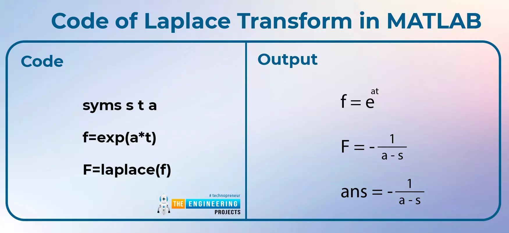
Here, you can see that the long calculations and formulas are condensed into a simple program of just three lines, and we get the correct output easily. Let’s understand this code. 

• First of all, we declared the variables that we are going to use in our Laplace transform. For this, we use syms. Any string after this is declared as a variable. If we do not do this, MATLAB will show an error and say that it does not have any information about that particular variable. 

• In the second step, we specified the equation of the question. In MATLAB, the exponential function is defined by using the exp(x) in which the x is the value that comes in the exponential area of the equation as you can see in the question. We stored this value in the variable f. You can use any value. 

• In the last step, we used the formula for laplace as it is a pre-defined function of MATLAB. In the equation, we just put in the value of the question that we had stored in the f. As a result, MATLAB will easily provide you with the answer and you do not have to go into deep calculations. 

 Enjoyed this example? Let’s move to a complex one. 

Code:

syms t u a

f=u*sin(a*(t-2))*(t-2)

F=laplace(f)

Output:

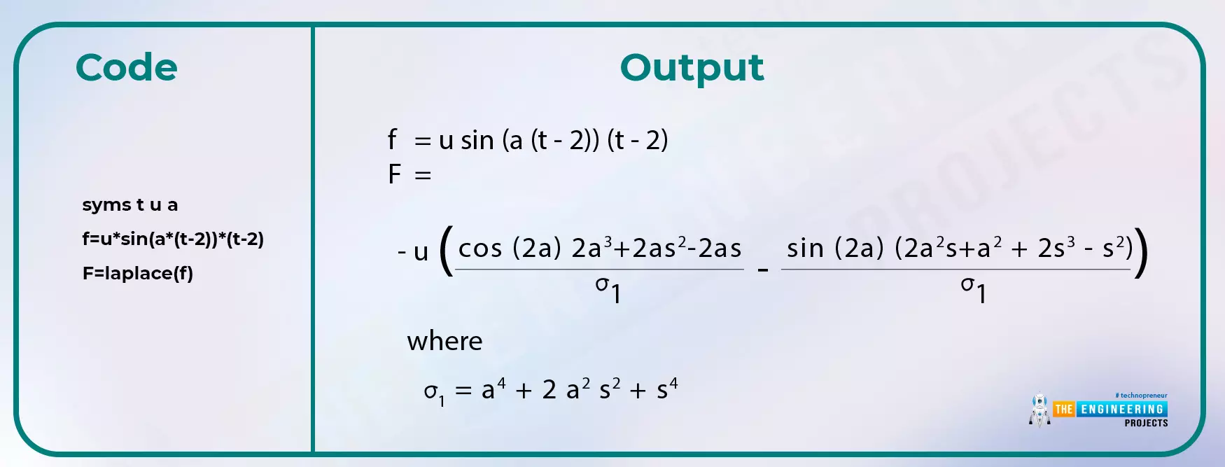
You can see the same procedure is followed by us in this example. We put a little complex equation in f and got the results as expected. The great thing is, that MATLAB provides us with the value of each term on its own without demanding us to clarify its answer. Always keep in mind that:

• There is a difference between capital and small letters. That is, MATLAB is case-sensitive. 

• The variable in which you store any information does not need declaration at the start but if you are using the variables in the equation, you have to specify them first so that MATLAB can distinguish them from the other variables and use them in the equation. 

It is important to understand the sequence in which we are going to study the Laplace Transform because the things are linked with each other, and at a point, you will feel that is why you are learning so much about that point, and after that when you learn the application of that particular thing, you will have the idea of that point. 

The Laplace transform can be solved with the help of a table that we will learn with great detail, and to understand that table, you have to have clear initial concepts. This table contains the properties of the Laplace transform that we’ll discuss in detail in the next session. 

Bilateral Laplace Transform

Here is a different way to solve the Laplace transform. Recall that the Laplace transform that we have read about till now is unidirectional; that is, the limits of the integration start from zero to positive infinity. Yet, now we are dealing with another type of Laplace transform that has a total limit. Yes, you are right, the limits of the integration are from negative infinity to positive infinity, and, therefore, it behaves differently from the one that we have discussed before. Here, we are denoting the Laplace transform with different variables so that it will be easy for you to memorize the difference in the behavior.

This type of transform is also known as the two-sided Laplace transform. Having a greater range of integration, this transform works a little differently.

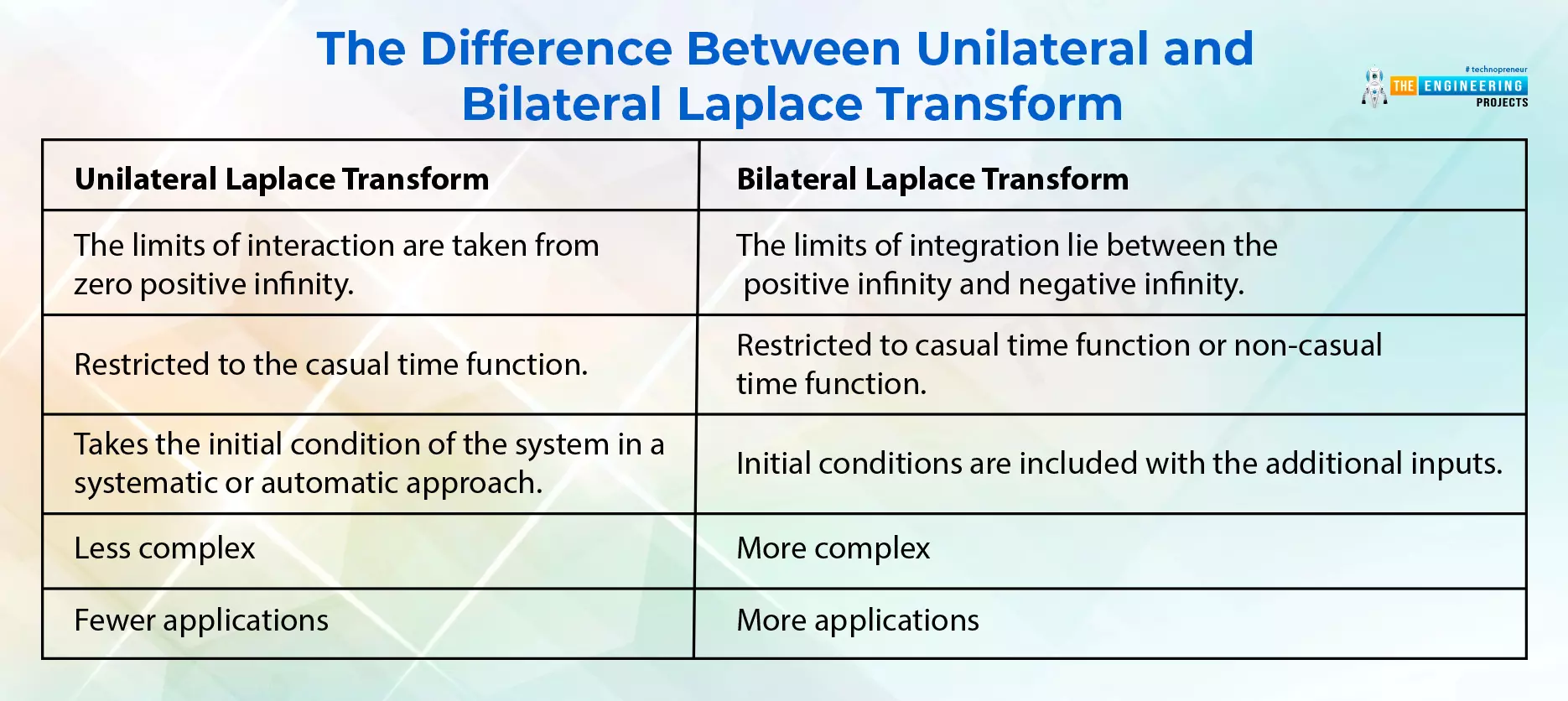
The Difference Between Unilateral and Bilateral Laplace Transform

People dealing with the practical applications of signals and systems have deep experience with both of them, and they use both of them in their work according to the nature of their work. Both of these have their own pros and cons, but once you have a clear concept of the unilateral Laplace transform, you can easily understand the other type.

So today we started an important topic in signals and systems named “Transforms” and studied the introduction to the Laplace transform. We saw some codes in MATLAB, as an example, and also read about the difference between the bilateral and unilateral Laplace transforms. The next lecture is going to be full of action and will see some applications of transforms as well.