Properties of Convolution in Signals and Systems with MATLAB


Hey geeks, welcome to the next article of this series on signals and systems. In the previous lecture, we saw the basic types of convolution and learned about convolution in MATLAB. This time, we are going to enhance some concepts about it by learning about the properties of convolution and by adding some important pieces of information about the same topic. Have a look at today’s concepts:
What are some basic properties of convolution?
What is the correlation?
Discuss some types of correlation and their implementation in MATLAB.
What is the difference between convolution and correlation?
How convolution is used in different areas of science and how different departments are using this technique to control the parameters efficiently.
The Properties of Convolution
Once you have a clear idea of linear/circular convolution, you can easily understand its properties. These convolution techniques that we have discussed till now are used in many fields of signal processing, and if you have a grip on their concepts, you can easily use it anywhere they are applicable.
There are three main properties of linear convolution:
Commutative property
Associative property
Distributive property
Commutative Property of Linear Convolution
This property says that linear convolution is commutative. It means that no matter what the sequence of the signal or function is that is involved in linear convolution, the result will remain the same.
Mathematically,
x(n)*h(n) = h(n)*x(n)
It means whether you convolve the second function and multiply it with the first one or vice versa, the result will remain the same.
The Associative Property of Linear Convolution
We can replace a succession of Linear-Time Invariant systems with a single system pulse response that is equal to the convolution of the impulse responses of the individual LTI systems using the associative property of convolution.
Mathematically,
y(n) = [x(n)*h1(n)] *h2(n) = x(n)*[h1(n)*h2(n)]
This property implies when there are more than two signals involved in convolution.
The Distributive Property of Linear Convolution
This property also depends upon more than two functions. It is a combination of addition and convolution of the signals. It says that the result of the addition of two signals and then convoluting them with the third one is equal to the addition result of the convolution of each signal separately from the third signal. If it is not clear to you with this statement, have a look at the equation.
Mathematically,
x(n)*[h1(n)+h2(n)] = [x(n)*h1(n)] +[x(n)*h2(n)]
Correlation
Correlation is the measure of similarities between two signals, functions, or waveforms that are usually used in signal processing. In other fields of science, a correlation has other meanings. Yet, in signals and systems, correlation compares two signals and provides the similarity. It is introduced as:
“In signals and systems, correlation is the procedure to find the similarity between the values of two signals, and it also measures the extent of this similarity in such a way that zero correlation means no similarity and vice versa.”
This is an important procedure, as in signals and systems, all the work is done with the help of waveforms or signals, and correlation helps to figure out the extent of similarity between them.
The Formula of Correlation
Let’s take two signals out of one is x(t) and the other is y(t), then the correlation, denoted by r, is obtained by using the following formula:
rxy(τ)= ∫∞−∞x(t)⋅y(t−τ) dt
Keep in mind that there is a difference between the relation of x to y and y to x. Therefore, changing the position with the r means we have to change the values on the other side of the equation as well. As you can see, the correlation is done by using the dot sign between the signals.
If you have the idea of convolution that we discussed in the previous lecture, then you must be familiar with the other components of the formula as well.
Types of Correlation
Based on how the correlation is solved in different ways, the correlation is broadly divided into two different types:
Autocorrelation
Cross-correlation
Autocorrelation
The first type of correlation is the one in which the signal is compared with itself. Here is the formula for it:
rxx(τ)=∫∞−∞x(t)x⋆(t−τ) dt
Now the question arises, how can a signal be compared with itself to find the similarity? Well, as you can see clearly in the formula, the signal x is correlated with the time-shifted version of the signal itself. In this way, we can say, auto-correlation is a uni-signal procedure.
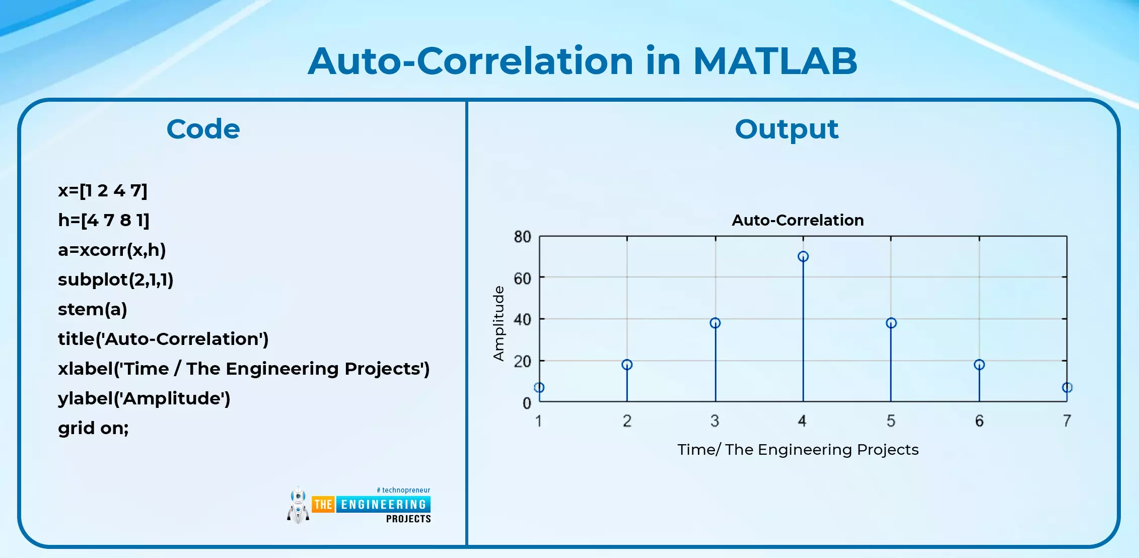
Auto-correlation in MATLAB
Code
x=[1 2 4 7]
h=[4 7 8 1]
a=xcorr(x,h)
subplot(2,1,1)
stem(a)
title('Auto-Correlation')
xlabel('Time / The Engineering Projects')
ylabel('Amplitude')
grid on;
Output
Cross-Correlation
The measure of similarity or coherence between one signal and the time-delayed version of another signal is defined as the cross-correlation between two different signals, functions, or waveforms. The degree of relatedness between one signal and the time-delayed version of another signal is indicated by cross-correlation.
Cross-correlation in MATLAB
Code
t=2:0.1:1
x=[1 2 4 7]
h=[4 7 8 1]
a=xcorr(x,h)
subplot(2,1,1)
stem(a)
title('Correlation')
xlabel('Time / The Engineering Projects')
ylabel('Amplitude')
grid on;
Output
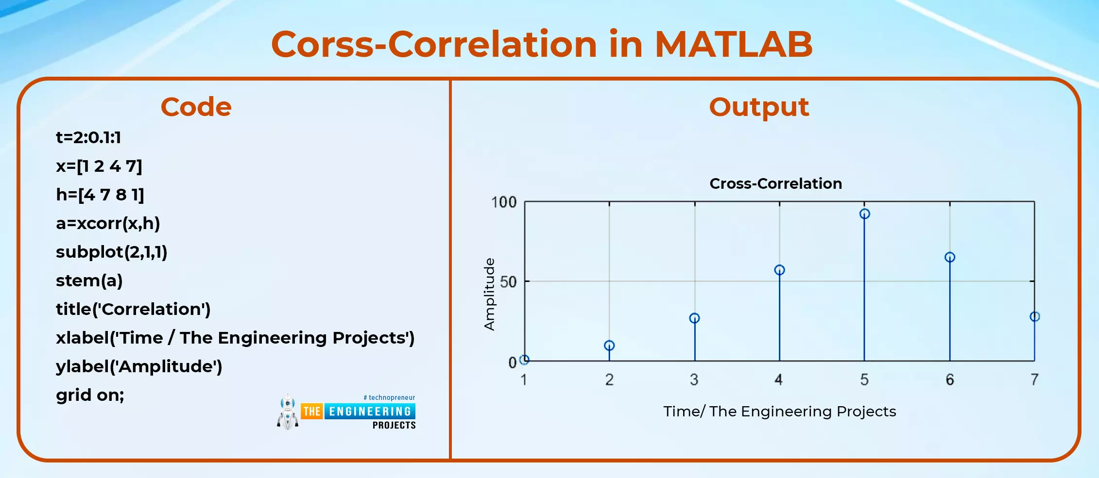
You can see it is a simple program with two signals and by using a simple formula of correlation as:
xcorr(i,j)
Where i and j are the signals, we can have an accurate correlation between the signals. There are some cases in which more than two entries are possible in the same formula, and MATLAB works best in that too.
Always keep in mind that we are using the stem command to show the signal in the discrete format, but you can also have the results in the continuous time format by simply putting the value of the result (here a is the result) in the plot format to get the desired result.
The Difference Between Convolution and Correlation
Convolution |
Correlation |
|
Introduction |
Overlapping two signals to have the third one. |
Finding the relation between two signals |
Denotion |
It is denoted by a (*) sign between signals |
It is denoted by a dot (.) between signals. |
The number of signals |
Always two or more |
Maybe 1 or more |
Types |
Linear convolution, circular convolution |
Auto-correlation, cross-correlation |
Functions in MATLAB |
conv(a,b), cconv(a,b) |
xcorr(a,a) ,xcorr(a,b) |
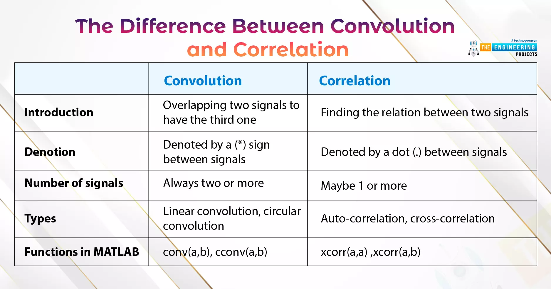
You will also see some other differences between these two at some points, but according to the point of view of the course we are studying, these applications are more than enough to understand. It is an important question that is usually asked during exams, and you must go through each of these points to clear up the concept.
Applications of Convolution
As we have said earlier, convolution is an important topic in signals and systems. Now, we are moving toward its applications so that you will get an idea of why we were emphasizing the importance of this topic. Here are some important and interesting applications of convolution techniques in signals and systems.
Image processing
Customizing patterns of signals
Audio processing
Polynomial multiplication
Artificial intelligence
Optics
We are going through each of these points consecutively because if you are familiar with the convolution technique as we have given the details in the previous sections, you are going to enjoy each of these. We are not going deep into the discussion because the deep discussion is not in the context of this course. You just have to understand the information and you will be amazed to know how simple topics can be useful in different ways.
Image Processing Techniques
First of all, let us discuss the way in which convolution changes the quality of the picture in any way you want. To understand it well, let’s discuss some points.
Image processing is based on tiny pixels, and the number of pixels decides the quality of the picture.
Operations on the images in a computer system are processed in the form of 2D arrays.
The processing of images is done by using matrices of different sizes, and the smaller one is called the Kernal, and its size is important in this process. Through the convolution process, we can change the edge privilege (as shown in the picture), and in this way, we can change the edge style with this technique.
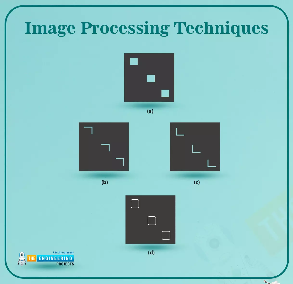
In the same way, convolution is used to sharpen or smooth the image according to the requirements. Another application of convolution in image processing is to blur the image to maintain the security or any other intention behind the convolution.
Customizing the Pattern using Impulse Response
As we have mentioned in the theoretical section before this, we can deal with the impulse response of the signals in convolution and if a person has deep knowledge of it, he can customize the pattern effectively using signals according to their own choice.
Audio Processing using Convolution
Similar to image processing, audio processing can also be controlled with the help of this technique. Audio signals can be mixed to have the third one, or you can simply use them to enhance the quality of your sound signals.
"Convolution reverb" is the technical term for the process of digitally simulating reverberation. It allows you to convolve the known impulse response of an area with that of the desired sound to simulate the reverberation effect of a specific area.
Multiplication of Polynomials
You have probably seen the multiplication of polynomials in your early classes, and you must be wondering why we are mentioning this term here. Keep in mind that polynomials may be very complex at a high level and it may become a headache to solve them correctly. Luckily, convolution can solve such multiplication within seconds by converting these polynomials into a matrix and solving them accordingly. In the end, when we have the values of each polynomial, one can also use the calculation further to use them for other purposes. Have a deep look at our description. We are talking about the multiplication of polynomials, but in real life, the convolution is carried out instead of multiplication, and we get the desired results.
Artificial Intelligence and Convolution
Convolution are used in artificial intelligence and e all now it is an emerging technique in which many people are working. Artificial intelligence works by using different types of networks of elements, and these networks are associated with the parameters that are known as “weight”. These weights are somehow associated with the convolution process, and in this way, we can change the influence of a particular node at a particular output.
Convolution in Optics
In the field of optics, where the major function is with the help of light and small details matter a lot, convolution is an effective way to change the parameters through which light is controlled. In this way, experts know how to control the light with the help of convolution.
The diffraction pattern in optics depends mainly upon two types of patterns of light:
Slits
Circular shape
And by carefully controlling these two parameters through convolution and other techniques, experts are doing great in the field of optics.
It was an interesting lecture today where we learned some important properties of convolution and gained a piece of great knowledge about correlation as well. For me, learning about the application of convolution was an interesting way to highlight the importance of my learning. You must go through some other points on the same topics as your homework. Now we are moving towards a relatively complex topic but do not worry, we are going to learn this step by step by mentioning all the basic and necessary information. In the next lecture, you will come across some different types of transforms in signal and system processing, and you will understand these if you have a little information about the time domain and frequency domain. So go through these, and have a great day.