Properties of Fourier Transform in MATLAB


Hey, pupils welcome to the next session about the Fourier transform. Till now, we have learned about the basics of Fourier transform. It is always better to understand all the properties of a mathematical tool to understand its workings and characteristics. You will observe that most of its properties are similar to the topics that we have discussed before, and the reason is, that all of them are transforms, and the core objective of these transforms is the same. We have learned about the simple and easy discussion of the Fourier Transform, but when dealing with complex problems, it involves the usage of different properties so that we do not have to repeat the calculations all the time to get the required results. Have a look at what you are going to learn today:
What are the basic properties of the Fourier transform?
How can you ding the inverse Fourier Transform?
How to implement inverse Fourier transform in MATLAB?
What are some applications of the Fourier transform?
So let’s start with the properties of this transform.
Linearity
First of all, the Fourier transform is linear. It means if we have two expressions of the Fourier transform that are denoted by G(t) and H(t) then combining them with the help of mathematical operations such as multiplication or addition results in an expression that is also linear.
Duality
It is an attractive property of the Fourier transform that says when a discrete-time signal is transformed into the frequency domain, then it can be regenerated into its time domain form by multiplying it with a negative factor, but in this way, we will get the reverse of the original signal.
Modulation of the Fourier Transform
The modulation of the Fourier transform occurs only when both the signals, that are to be modulated are in the form of functions of time.
Time Shifting Property of Fourier Transform
This property of Fourier transform says that if we are applying it on a function g(t-a) then it has the same proportional effect as g(t) if a is the real number. If you have a clear idea of the procedure of time scaling, it will be easy for you to understand the situation here.
Parseval’s Theorem of Fourier Transform
This theorem is related especially to the Fourier transform. It says that the sum of the squares of a function x(t) is equal to the Fourier transform of the function x(t).
It is an important theorem because once we have this clear theorem, we do not have to calculate the square of the whole series of Fourier transforms. So, it becomes easy to deal with these quantities with the help of this theorem.
Scaling in Fourier Transform
Scaling of the signal is the process in which there is a change in the independent variable or the data features in the form of a range of the signal. This property says that if the values of the signals on the x-axis in the time domain are inversely proportional to the values on the x-axis when we convert them into the frequency domain. In other words, the more stretched a signal is in the time domain means less stretched and a taller signal in the frequency domain and vice versa.
If
f(t) = F(w)
Then,
f(at) = (1/|a|)F(w/a)
Convolution in Fourier Transform
Convolution is the process in which two signals are overlapped on each other in such a way that we obtain a third signal that is different from the first two. When we talk about the convolution of the two signals, we get results that are equal to the convolution of the same function in the Fourier transform.
Mathematically,
If
f(t) = F(w) and g(t) = G(w)
Then,
f(t)*g(t) = F(w)*G(w)
In this way, it becomes easy to predict the result if we know the value of one function and are interested in knowing the other.
Differentiation of the Fourier Transform
We all know the procedure of differentiation, and when we are differentiating the Fourier transform, we may get confused about following the rules of both these procedures. So, with the help of using this property, you can easily guess the results. This property says that:
If
f(t) = F(w)
Then,
f'(t) = jwF(w)
Where j is the variable and w is the function based on which the differentiation is occurring.
Inverse Discrete Fourier Transform or DFT
So far, we have learned how DFT is used to obtain the signal in the frequency domain. But what if we want the inverse results? What if we want our original signal back? Well, it is the requirement of a large number of applications, and then the inverse Discrete Fourier Transform is used. It is not a new concept to use the inverse methods, as we have also read it when we were discussing the previous transforms.
To perform the inverse method, we just have to simply follow the formula given below:
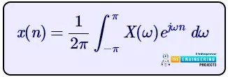
All the other variables are the same. We just have to remember the formula and we are good to go.
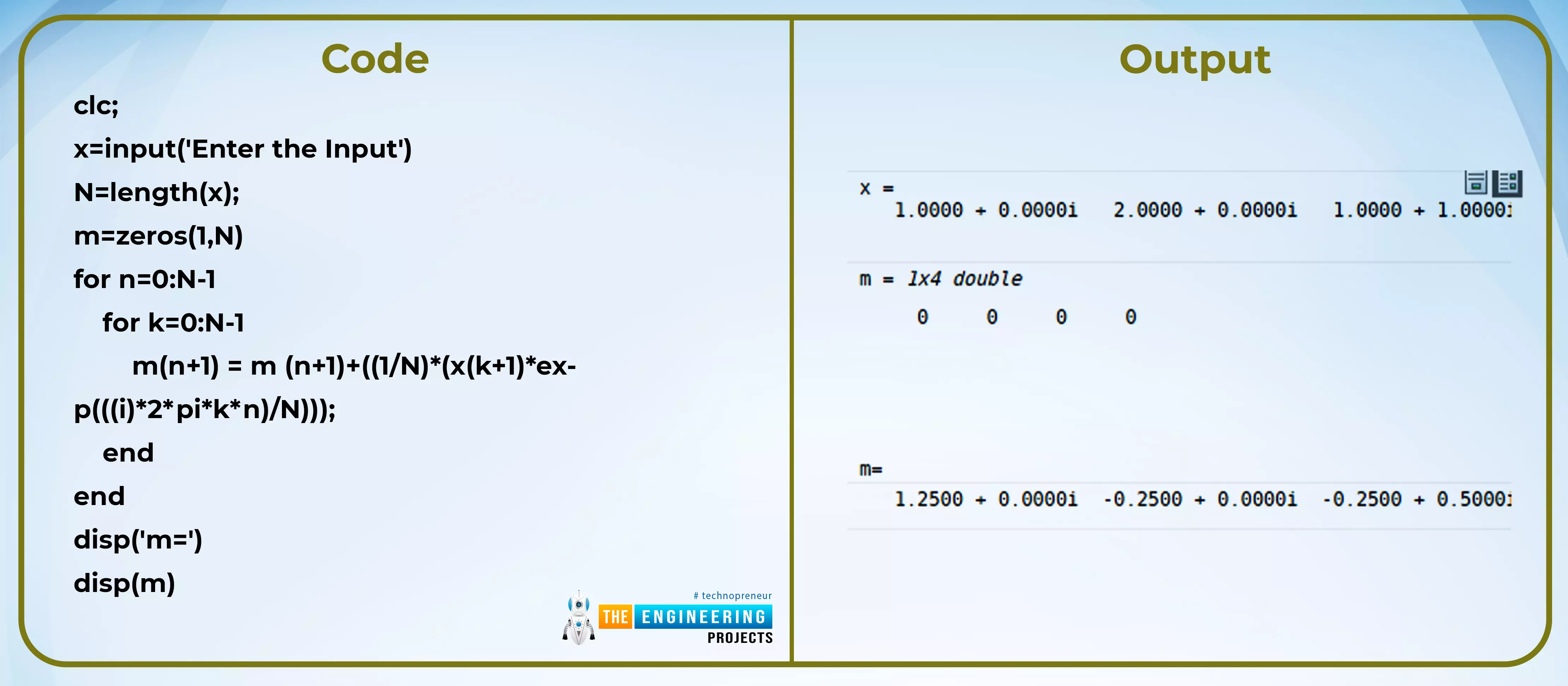
Code:
clc;
x=input('Enter the Input')
N=length(x);
m=zeros(1,N)
for n=0:N-1
for k=0:N-1
m(n+1) = m (n+1)+((1/N)*(x(k+1)*exp(((i)*2*pi*k*n)/N)));
end
end
disp('m=')
disp(m)
Output:
Let’s understand this code. There are a few things that we have used for the very first time in this series, and therefore, I want to describe them all.
clc; in MATLAB
It is a very common and useful command that you will often see in the first place of almost every MATLAB code. The purpose of using this line is to clear all the data that you are looking at on the screen of your display window.
There is a window just below the working area of MATLAB called the “command window." main reason why we are discussing this line here is that we have not used the input function till now in this series, and therefore, I do not feel any need for this clear screen command here. This will be more clear when you learn about input functions.
Input Function in MATLAB
In MATLAB, when we want to input the values of a particular quantity on our own, we use the following function:
input(x)
Where x is the quantity that we want to have the input of. Moreover, you can also use it to provide the statement on your own (as we have done in our program), but the statement should be enclosed in inverted commas if you want to print the statement as it is.
disp(x) in MATLAB
This is another function that we have used for the first time in this series. Well, this is the display function, and it is used to display the result or quantity that we want. Here in this code, for instance, we wanted to show the value of the result that we have stored in “m”. Therefore, we first displayed the m in inverted commas so that it was printed as it was, and after that, when we used the same function without the inverted commas, we got the value of the m that was stored before.
For Loop in MATLAB
Loops are used in many programming languages, and if you have the basic concepts of programming languages, then you must know that “for loops” in MATLAB are used when we want that compiler to stay at a particular line and repeat the same line until a particular condition is fulfilled.
In our case, we started the first loop when m=0 and it stayed at that particular line till the value was one less than N. The same case was with the second loop. Once the condition was met, the compiler moved toward the next line.
The syntax of the for loop in MATLAB is:
for x:y
Statement
end
Where x is the starting point of the for loop and y is the ending point of the for loop, both of these are specified by the programmer, and a statement is a calculation that we want to perform again and again.
Explaining the Code of IDFT in MATLAB
Clc clears the screen of the command prompt in case you are using the code for the second or more time.
The input function displays a message to the user that input is required from him/her.
The input by the user is stored in the variable x.
Now, we are introducing another variable, m, that stores the result calculated by the length function. It is the total number of values provided by the user.
Here, we are calculating the number of zeros between the number 1 and the length of the input by the user that was stored in N.
The interesting part starts here. We are using two for loops, which means we are nesting the loops. The condition of both of them has been discussed before. The formula that we have hardcoded inside these loops is used till the conditions provided by us are met. To perform the functions on the series of signals, loops are used in this way so that we do not have to write the same lines again and again.
In the end, when we have the results stored in the variable m, we just display it with the label m, and our program is completed.
Applications of the Fourier Transform
As we have mentioned that Fourier transform has great importance in many fields of education and science and therefore, great work has been done by using this technique. Some important fields and applications of the Fourier transform are discussed in this section.
Fourier Transform in Medical Engineering
In medical engineering, where we get complex and hard results. The Fourier transform is an old technique and therefore, it is used in the field of medical engineering for a long time. The impulse response and delicate results in the form of the signal are fed into the compilers where these signals are tested and examined deeply in a better way.
Fourier Transform in Mobile phones
Here is an interesting application of the Fourier transform. We all know that cell phones work with the help of signals and therefore, there is a lot of work that can be done by using the Fourier transform. If you are wondering how the Fourier transform is performed in the cell phone then you are at the right point. Actually, while making, testing, and designing cell phones and other such products, the rules and calculations of Fourier transform are used widely because of its precise result and research.
Fourier Transform in Optics
As we discussed from the beginning, the Fourier transform works great with the signals. The optic is the field that works in the waves and delicate signals and therefore, the Fourier transform is used to sum all the results in a great way and to find the results according to the need. Most of the process occurs in the optics when the light or other rays are merged into one point, and with the collaboration of other techniques, the Fourier transform works great to make all the procedures easy and accurate. Moreover, the Fourier transform is also useful for the smoothness of the signals and filtering of the results as well.
So, today we learned interesting information about the Fourier transform, and now we can say that we have all the basic information about the Fourier transform. We have seen the properties of the Fourier transform and also learned about the inverse Fourier transform, along with the MATLAB code for a perfect concept. The concept of the for loop, clc, and input method was new to us. In the next session, we are going to talk about the comparison of all these transformations. So be with us.