Basic Operations on Signals in MATLAB


Hey peeps welcome to The Engineering Projects. This is the third lecture of this series, and till now, we have discussed the introduction to the signal and system, and in the previous lecture, we learned about the classification of signals and the difference between some of them.
In the present day, you are going to learn the basic operations of signals, and it is amazing to note how you can play with these signals. The best thing about this series is that you are going to see every step with the help of MATLAB. Let’s have a quick glance at today’s topic, and after that, we will go through a detailed explanation.
Addition of Two Signals
Subtraction of Two Signals
Multiplication of Two Signals
Time Scaling (Compression and Expansion)
Time Shifting (Addition and subtraction)
Reversal of Signal
Moreover, you will also learn some practical applications of some of these operations. All these operations are explained with the help of MATLAB code, and for simplicity, the codes are kept basic so that you may learn more about the concepts.
Basic Concept
Keep in mind that a signal has some parameters on the basis of which its graphical representation gets a face. These parameters are
Time
Amplitude
In all the operations, we will deal with these two parameters and change their values in different ways. Recall in mind that the greater the amplitude, the longer a signal goes on the y-axis and more time means that we’ll get wider loops of the signals. Time is an independent quantity and it is always kept on the x=axis no matter what type of signals are you dealing with. In each signal, when working on MATLAB, you will put the time in the first place from the left when using the Stem or Plot function.
Operations on the Signals
Addition of Signals
We are starting with the easiest operation of the wave. The addition of the signal is the process in which the amplitude of two signals is added and as a result, the signal obtain has the combination amplitude of both of these. The simplest example of this operation is:
x1=sin(2πt)
x2=cos(2πt)
y=x1+x2
The resultant Y has the value of the addition of both these signals. Have a look at the same result on MATLAB for the best graphical representation.
MATLAB code for Addition of Signals
Code |
Output |
t=0:0.01:0.1 f=25; t1=2*pi*f*t; x1=sin(t1); subplot(3,1,1) plot(t,x1) title('x1') grid on; x2=cos(t1) subplot(3,1,2) plot(t,x2) title('x2') y=x1+x2 subplot(3,1,3) plot(t,y) title('y= x1+x2') xlabel('Time/ The Engineering Projects') ylabel('Amplitude') |
|
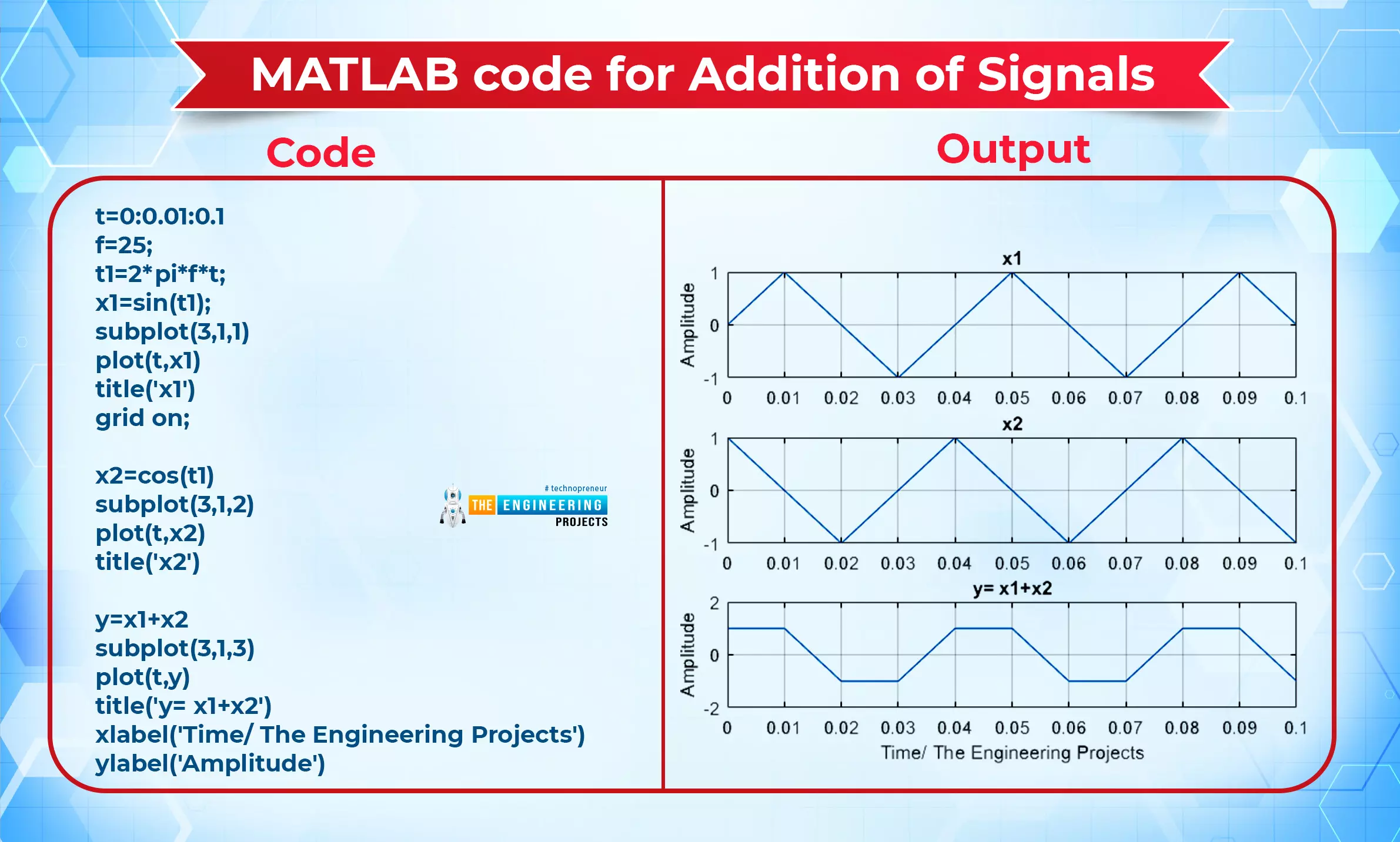
Keep in mind, this is not the amplitude at which the operation of addition takes place but the values of the amplitude are summed up and MATLAB store these values and show you another wave of this. You can match the values of the result from the workspace window or simply have a look at the wave. Let’s start from the initial point:
y=x1+x2
At point 0
1=0+1
At point 0.01
1=1+0
At point 0.02
-1=0+(-1)
And so on.
Subtraction of Signals
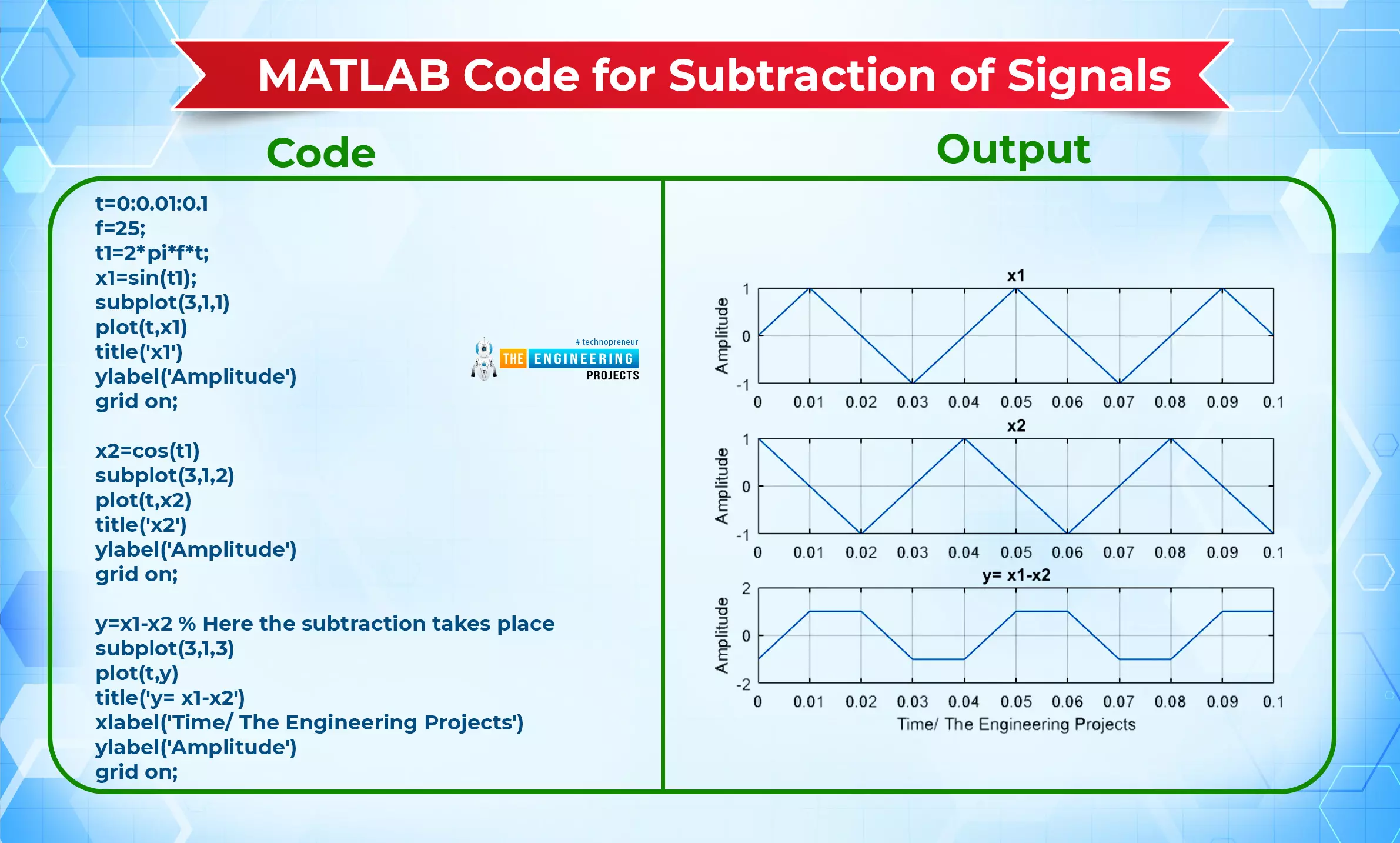
Subtraction is also possible in the signals, just like the addition operation. Subtraction between the two signals takes place when the value of the second signal (the one that is written after the subtraction sign) is subtracted from the first signal.
In MATLAB, for simplicity, we are using the same code with the value of subtraction between x1 and x2.
MATLAB Code for Subtraction of Signals
Code |
Output |
t=0:0.01:0.1 f=25; t1=2*pi*f*t; x1=sin(t1); subplot(3,1,1) plot(t,x1) title('x1') ylabel('Amplitude') grid on; x2=cos(t1) subplot(3,1,2) plot(t,x2) title('x2') ylabel('Amplitude') grid on; y=x1-x2 % Here the subtraction takes place subplot(3,1,3) plot(t,y) title('y= x1-x2') xlabel('Time/ The Engineering Projects') ylabel('Amplitude') grid on; |
|
Multiplication of Signals
Okay, you must think that this will be the same as the previous two concepts, but no. There is something different from the previous one, but before exploring that, let’s just define the multiplication of the signals:
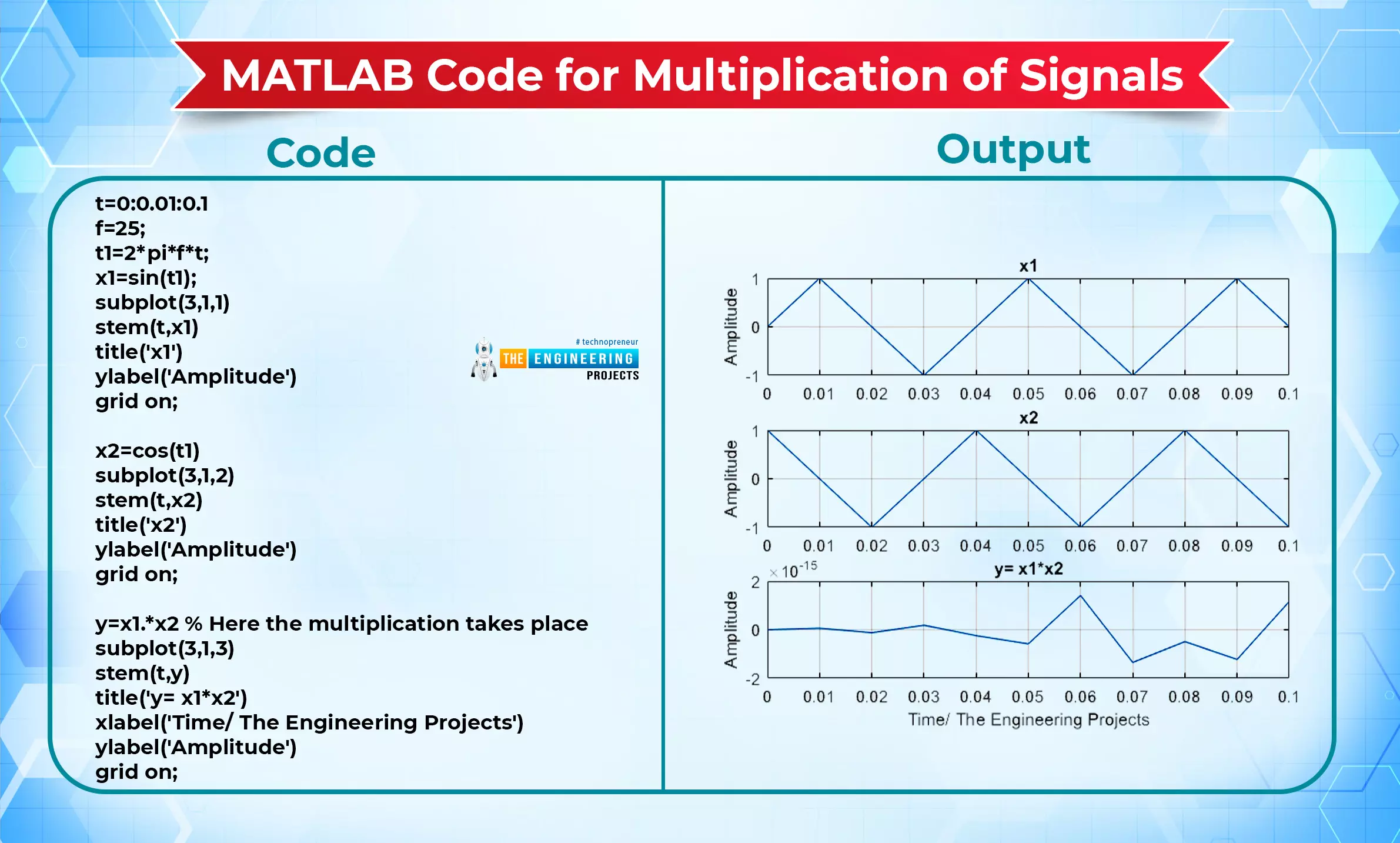
“The multiplication of two signals is obtained when the values of the amplitude of two signals are multiplied and the resultant signal has the multiplied amplitude.”
Have a look at the MATLAB code.
MATLAB code for Multiplication of Signals
Code |
Output |
t=0:0.01:0.1 f=25; t1=2*pi*f*t; x1=sin(t1); subplot(3,1,1) stem(t,x1) title('x1') ylabel('Amplitude') grid on; x2=cos(t1) subplot(3,1,2) stem(t,x2) title('x2') ylabel('Amplitude') grid on; y=x1.*x2 % Here the multiplication takes place subplot(3,1,3) stem(t,y) title('y= x1*x2') xlabel('Time/ The Engineering Projects') ylabel('Amplitude') grid on; |
|
Time Scaling of Signals
If you are new to signals and systems, this is something different that you will learn for the first time. At first, you may think that it is a simple multiplication of signals, but soon you will realize that only one signal is used in this operation, the opposite to the case that we have discussed earlier. Have a look at the definition of this operation:
“The term time scaling refers to the process of multiplying a constant by a signal's time axis. This technique is also known as time scaling of the signal."
Depending on the magnitude of the constant or scaling factor, the time scale of a signal has two possibilities:
Compress
Expansion
These two processes occur depending on the amount of time it takes to complete the signal.
Compression in Time-Scaling
Compression of the signal occurs when the constant number, multiplied by the signal is greater than zero and as a result, a signal is obtained that has a less wide form than the parent signal. It is because the time axis has more values in the resultant signal.
Expansion in Time-Scaling
You can say it is the opposite phenomenon of the compression of the signal. In this process, the constant number that is multiplied by the signal is less than zero, and therefore, the gained signal has a wider form.
When data is to be brought in at a certain rate and taken out at a different rate, the time scaling operation of signals is a highly helpful tool to have. It will be more clear when you will observe this example:
MATLAB code for Time Scaling of Signal
Code |
Output |
t=0:0.01:8*pi x=sin(t); subplot(3,1,1) plot(t,x) title('Simple Signal') xlabel('Time') ylabel('Amplitude') grid on; y=sin(t/2) subplot(3,1,2) plot(t,y) title('Expanded Signal') xlabel('Time') ylabel('Amplitude') grid on; z=sin(t*2) subplot(3,1,3) plot(t,z) title('Compressed Signal') xlabel('Time/ The Engineering Projects') ylabel('Amplitude') grid on; 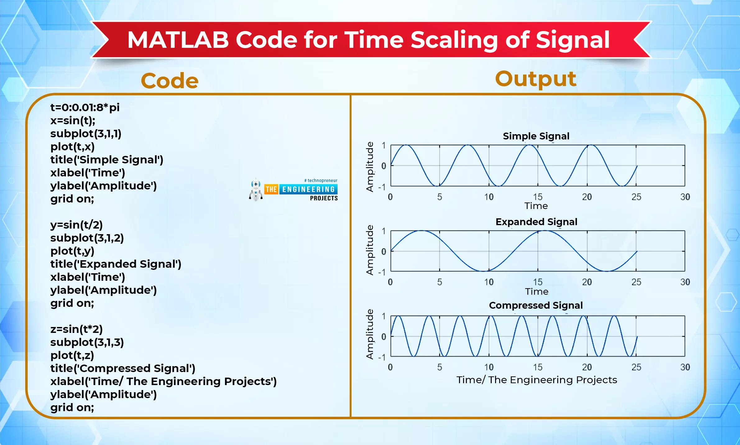
|
|
Applications in the Real World
Changing the rate at which the signal is sampled is the primary focus of the time scaling technique that we employ. Altering the frequency at which a signal is sampled is one technique that is used in the field of voice processing. A system that is based on a time-scaling algorithm that was built to read text to people who are visually impaired is a specific example of this.
Time Shifting of Signals
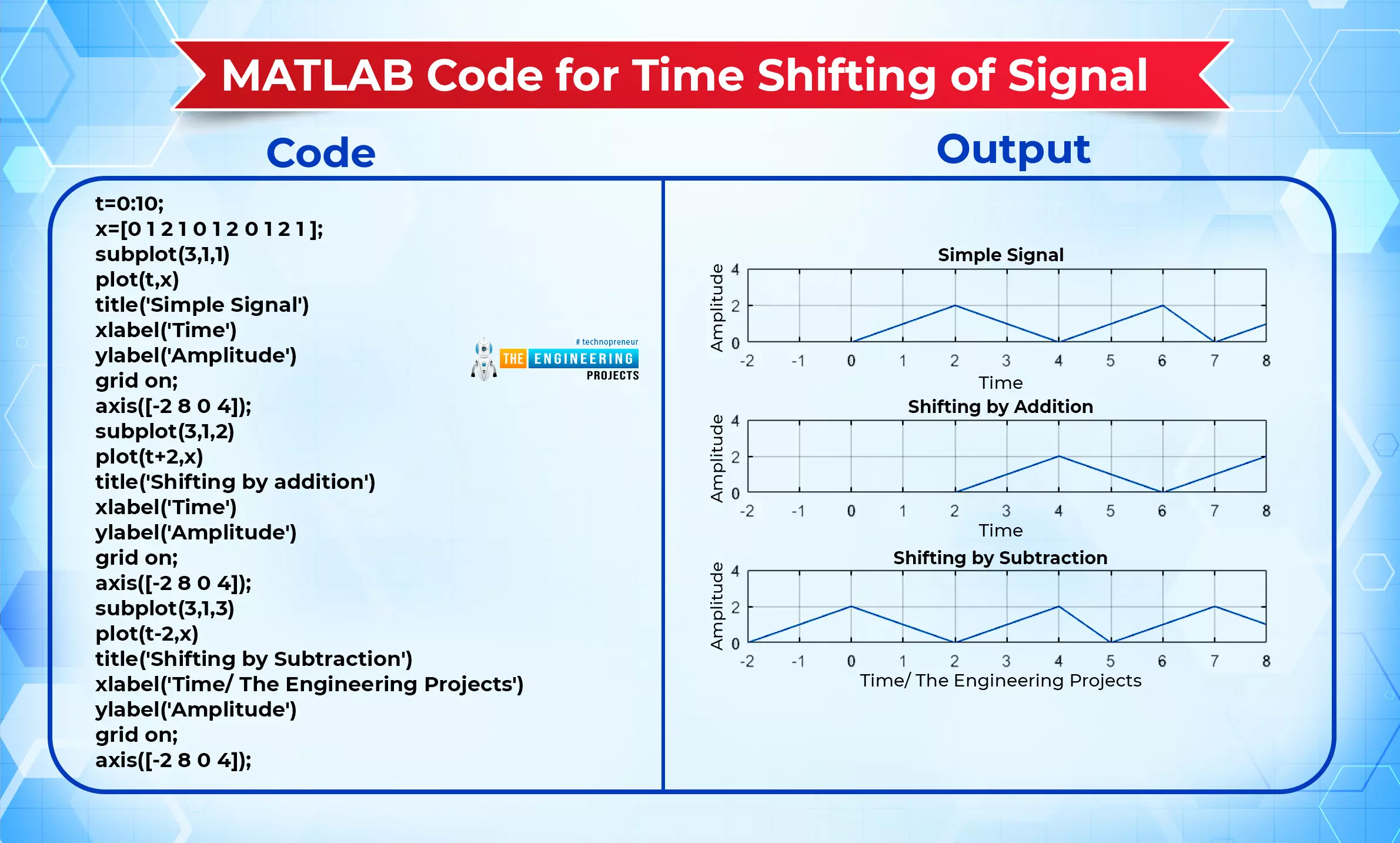
This is another operation on the signal in which the x-axis or time axis changes. Instead of changing the width of the signal, we are shifting the wave to a different location on the x-axis.
“The process of moving a signal forward or backward in time is what the term "time shifting" refers to. To do this, either an additional amount of the shift or subtraction from it is applied to the time variable in the function.”
It is interesting that you are moving the whole signal on the time axis. It has two processes:
Addition in Time Shifting
This process is used to move the whole signal to the right side of the time axis. The whole signal moves towards the right side and the amplitude does not change.
Subtraction in Time Shifting
As you can guess, by subtracting the value on the time axis, you can simply move your signals to the left side of the x-axis no matter where they are at the start.
MATLAB code for Time Shifting of Signal
Code |
Output |
t=0:10; x=[0 1 2 1 0 1 2 0 1 2 1 ]; subplot(3,1,1) plot(t,x) title('Simple Signal') xlabel('Time') ylabel('Amplitude') grid on; axis([-2 8 0 4]); subplot(3,1,2) plot(t+2,x) title('Shifting by addition') xlabel('Time') ylabel('Amplitude') grid on; axis([-2 8 0 4]); subplot(3,1,3) plot(t-2,x) title('Shifting by Subtraction') xlabel('Time/ The Engineering Projects') ylabel('Amplitude') grid on; axis([-2 8 0 4]); |
|
Applications in the Real World
A significant number of signal-processing applications make use of an operation known as time-shifting, which is an essential procedure. For the purpose of performing autocorrelation, for instance, a version of the signal that has been time-delayed is utilized.
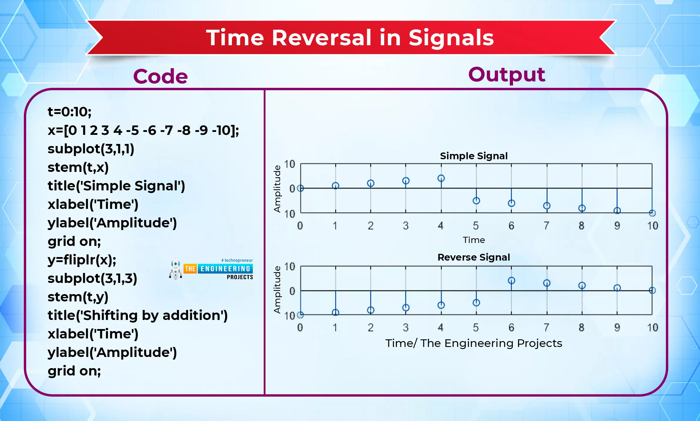
Time Reversal in Signals
When one is first learning about time scaling, one of the most natural questions to ask is, "What happens when the time variable is multiplied by a negative number?" Time travel is the solution to this conundrum. This procedure inverts the time axis, often known as flipping the signal over so that it reads along the y-axis.
“ The process of flipping the whole signal by using the flipping function or by multiplying the whole signal with a negative number is called reversal of the signal because each and every value of signals is reversed”.
This technique is useful in many cases, and the best thing is, that you do not have to change your code much. Just 1 step and you are good to go.
Code |
Output |
t=0:10; x=[0 1 2 3 4 -5 -6 -7 -8 -9 -10]; subplot(3,1,1) stem(t,x) title('Simple Signal') xlabel('Time') ylabel('Amplitude') grid on; y=fliplr(x); subplot(3,1,3) stem(t,y) title('Shifting by addition') xlabel('Time') ylabel('Amplitude') grid on; |
|
Conclusion
There are certain operations on the signals that are too easy to perform but have the ability to change the working of the entire signal. These operations work as the backbone of the signal and system, and once you have command of this, you can work more deeply with the signals. You may also see some other operations in the upcoming tutorial, but for now, you must practice these basic operations and try to make your own signals and play with them. It is an interesting task that must be done on the same day as you learn the basic definition of these signals.