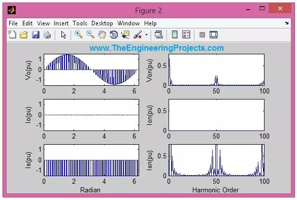
Hello friends! Today, we will analyze sinusoidal pulse-width modulation of an AC signal in MATLAB. We will generate a carrier, compare it with a reference, calculate a switched voltage and examine the resulting current and frequency spectrum. The aim is to understand what the equations mean rather than simply obtain a collection of plots. The original tutorial gates an existing sinusoidal supply on and off. That is an idealized AC-chopper model, which differs from a DC-fed inverter that synthesizes AC by switching a DC link. We will preserve that original idea and make the switching assumptions explicit so the calculated voltage, current and power factor describe one consistent circuit model. We will also correct several common analysis mistakes: confusing pulse count with period, treating ...
Hello friends! Today, we will discuss fault detection of a gas turbine in MATLAB and Simulink. The aim is to understand how measurements, a reference model and decision logic can work together to identify abnormal behavior. We will move from the physical system to residual calculations, then examine how to test a detector without confusing a simulated alarm with a validated machine-protection system. The original project contains a useful collection of scopes, delays, summing blocks and alarm indicators. However, some block names and explanations need correction. In particular, a mu-law signal compressor is not an air compressor, and a piston-engine power-stroke model does not become a gas-turbine model merely by changing its displayed name. We will retain the original screenshots as a his ...
Hello friends! Today, we will learn how to create a GUI in MATLAB. GUI stands for graphical user interface: a window containing controls such as buttons, text fields and plots that let someone operate a program without typing every instruction in the Command Window. Our first application will be deliberately small so that we can understand what happens behind each control. We will enter a message, press Start and display that message elsewhere in the window. Although this sounds simple, it introduces the same important ideas used in larger engineering applications: reading input, responding to an event, validating data and updating an output. Once these steps make sense, adding a calculation or graph becomes much easier. This article originally used MATLAB's GUIDE editor. We will preserve ...
Hello friends! Today we will send data from MATLAB to a serial port. We will begin with one character, then send a line of text entered by the user, and finally look at binary bytes, replies and connection cleanup. These are useful building blocks when a MATLAB calculation needs to communicate with an external instrument or microcontroller. The original tutorial used MATLAB's older serial object. That code remains useful for understanding historical projects, but modern MATLAB code normally uses serialport. We will explain both interfaces clearly so that you do not mix their connection and writing functions in one program. Before connecting any actuator, start with a receiving terminal, a suitable loopback arrangement or a device command whose effect you understand. Seeing a message in MAT ...
Hello friends! Today we will study multilevel inverters, starting with the switching waveform and then looking at the circuits that produce it. An inverter converts electrical power from a DC source into an AC output. Its switches determine the instantaneous voltage, while the modulation, load and filter determine how closely the useful output follows the required sine wave. In our earlier tutorials on pure sine wave inverter design and modified sine wave inverters , the main question was how to generate the alternating waveform. Here we will introduce intermediate voltage steps and examine what they change. More steps can improve waveform quality, but they also introduce more devices, measurements and control decisions. We will compare cascaded H-bridge, diode-clamped and flying-capacitor ...
Hello friends! This tutorial continues our financial calculations in MATLAB project. We will move from expected returns and covariance to portfolio allocation, performance measurement and a complete Black–Litterman update. The central idea is to begin with a reference portfolio and the returns implied by it, then combine those returns with explicitly stated views. We must also describe how uncertain the views are. A bar chart of implied returns alone does not complete the Black–Litterman calculation. We will retain the original project's teaching sequence and historical figures while correcting its treatment of backtesting and portfolio risk. The numerical example below uses hypothetical assets and assumptions for learning. Information about the earlier implementation remains on the origin ...
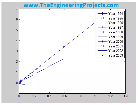
Hello friends! Today, we will work through financial calculations in MATLAB, beginning with historical market data and ending with portfolio risk-and-return plots. We will follow the original project's five stages: prepare the data, account for currency, calculate returns, estimate covariance and examine efficient portfolios. The original project compared seven market indices and explored a 3% risk-free-rate assumption. We will retain that framework, but correct several important details about exchange rates, rolling windows and portfolio interpretation. An expected return is an estimate, not a guaranteed result, and a graph is only as meaningful as the inputs behind it. This is an educational modelling example. The historical figures remain for context, while the formulas and code below e ...
Hello friends! Today, we will study a MATLAB project for modelling a DVB-T2 transmission system using consistent channel frequency responses. The main question is simple: when we compare two transmitter configurations, how can we make sure that a different random channel has not decided the result for us? We will follow the original project from its parameter-selection interface to its BER plots, then improve the experiment design through repeated trials and confidence intervals. Along the way, I will explain the difference between a channel realization and a received waveform, because confusing these two quantities makes a comparison unreliable. The original screenshots are retained as historical project results. Some settings and statistical labels in the earlier report were inconsistent ...
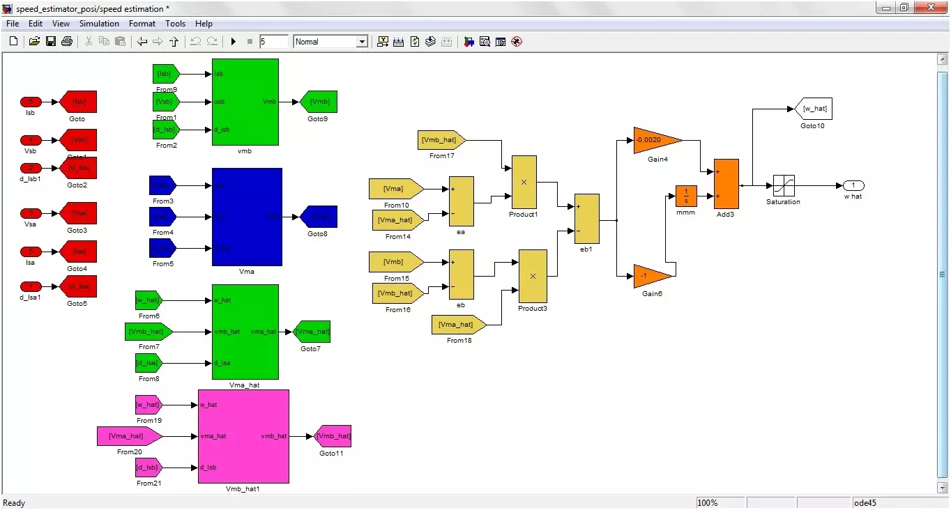
Hello friends! Today we will study sensorless speed estimation of an induction motor in MATLAB and Simulink. We will follow the original project's adaptive-estimation approach, beginning with the motor equations and then connecting those equations to the illustrated simulation blocks. The aim is to estimate rotor speed from electrical quantities rather than feed a measured shaft-speed signal into the estimator. In simulation, the motor model still provides a true speed for comparison. Keeping that reference separate from the estimator inputs is essential: otherwise, a model can appear sensorless while quietly using the answer it is supposed to estimate. The original project was developed in the MATLAB 2010 era and described as used with later 2012 and 2013 releases. The diagrams below docu ...
Hello friends! In this tutorial, we will find the roots of a quadratic equation in MATLAB, calculate its minimum over a specified interval and display the results on a graph. This is a useful beginner project because it connects algebra, functions, input validation and plotting in one small program. The original project allowed you to choose roots, a minimum or both. We will keep that idea, but make the calculations more reliable. In particular, we will distinguish a function's roots from its minimum, account for interval boundaries and handle inputs that turn out to be linear or constant. You do not need Symbolic Math Toolbox for the numerical program below. We will use ordinary MATLAB arrays, roots , polyval and a little calculus. Figure: MATLAB is used to calculate the polynomial roots ...