

Hello friends, today I am going to post a complete project designed on MATLAB named as Modelling of DVB-T2 system using Consistent Channel Frequency in MATLAB. This project is designed by our team and it involved a lot of effort to bring it into existence that's why its not free but as usual I have discussed all the details below related to it, which will help you understanding it and if you want to buy it then you can click on the Buy button shown above.
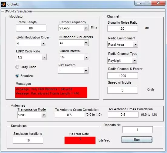
This project aims to implement a DVB-T2 (Digital Video Broadcasting for terrestrial television) system using consistent channel frequency responses. Tthe code is designed to use the same output from a channel model for different transmitter configurations so that consistency of performance results can be obtained. After that the overall project will be modified to repeat an experiment “n” times collecting data so that “x%” confidence intervals can be calculated. Historically, DVB is a project worked by more than 250 companies around Europe at first and now worldwide. DVB-T2 is the world’s most advanced digital terrestrial television (DTT) system, offering more robustness, flexibility and at least 50% more efficiency than any other DTT system. It supports SD, HD, mobile TV, or any combination thereof. The GUI for DVB-T2 parameters selection in MATLAB is shown on the left.
MATLAB Simulations & Results
DVB-T2 is the second generation standard technology used for digital terrestrial TV broadcasting. As it’s a new technology so it has many fields to explore and research, and the best way of researching on any new technology is via simulations. Simulations provide an easy and efficient way to evaluate the performance of any system. For simulation purposes, MATLAB software was chosen in this thesis because of its wide range of tools and ability to show graphical results in a very appropriate form. . Further, this DVB-T2 simulation model could be extended easily to simulate DVB-H, which shares many features with DVB-T2 (only the physical layer that needs modification). The most important feature, I discussed in my simulations are:
- Comparison of Bit Error Rate (BER) and Signal to noise Ratio (SNR).
DVB-T2 scheme can handle wide range of sub carriers from a range of 1k to 32k; these sub carriers can be fixed or mobile. In this thesis, experiments are performed on mobile transmission of signals to 4000 sub carriers. Below are discussed three different mobile scenarios, for different speeds of mobiles user, which are:
- Pedestrian moving at the speed of 0.1 km/h.
- Bus moving at the speed of 5km/h.
- Car moving at the speed of 10 km/h.
In all the scenarios, the factors mentioned below are kept constant so that a real comparison can be obtained and it could be checked that whether the speed affects the signal or not. These constant factors are:
- Transmission Mode is SISO.
- Transmitting Antenna Cross Correlation is 0.5.
- Receiving Antenna Cross Correlation is 0.5.
- Environment considered for these simulations is rural.
- Radio Channel type is Rayleigh with k factor of 1000.
- Carrier frequency is 91.429MHz.
1.1 Initial MATLAB model
During this thesis, help was taken from a MATLAB model of DVB-T2 transmission system designed by a student at Brunel University. First this initial model was studied and then enhanced it to a higher level. The first model designed by the student at Brunel University, performed the iterations on the DVB-T2 system and gives the results for just one cycle. Explanation of this initial model is discussed in detail below.
1.1.1 Explanation of Initial Model
After the user input all the values in the GUI, this model first calculates the below three values depending on the number of subcarriers attached to the DVB-T2 system.
- Useful OFDM period.
- Maximum number of sub carriers.
- IFFT / FFT length.
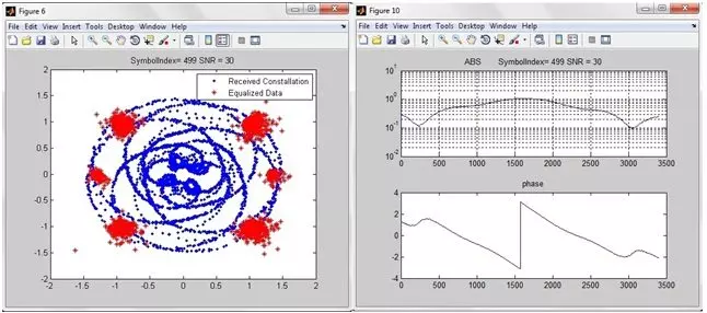
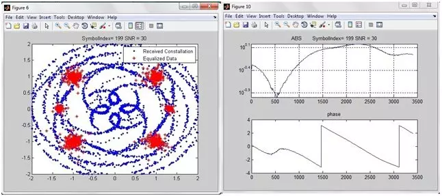
After getting this information, the model performs the QAM modulation over the signal so that it could be sent from the transmitter to the receiver. Next, depending on the value of Pilot Pattern given by the user, it calculates the scattered Pilot Amplitudes for the system. After that, it calculates the distortion in transmission depending on area in which the signal is propagating.
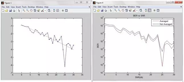
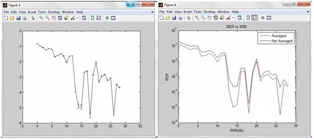
In order to calculate the distortion, FFT technique is performed on the signals to get their frequency response. As the signal has already sent from the transmitter after QAM modulation so demodulation on the receiver side is necessary. The model performs the same and demodulates the signal and finally it calculates the value of Signal to noise ratio (SNR) and Bit Error Rate (BER). At the end, it simply plots the graphs of SNR and BER for the visual representation.
1.1.2 Results of Initial Model
Different experiments were performed on the initial model and checked its results. The results are given below for three different experiments, which are:
- Speed of mobile = 0.1 km/s , Total Iterations = 5000
- Speed of mobile = 1.0 km/s , Total Iterations = 5000
- Speed of mobile = 10 km/s , Total Iterations = 5000
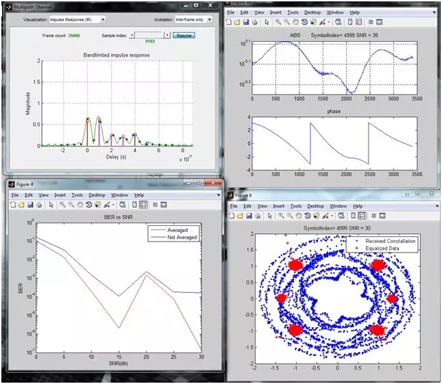
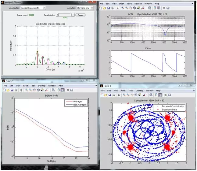
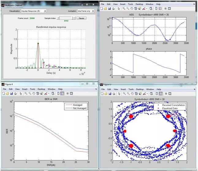
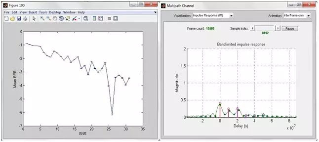
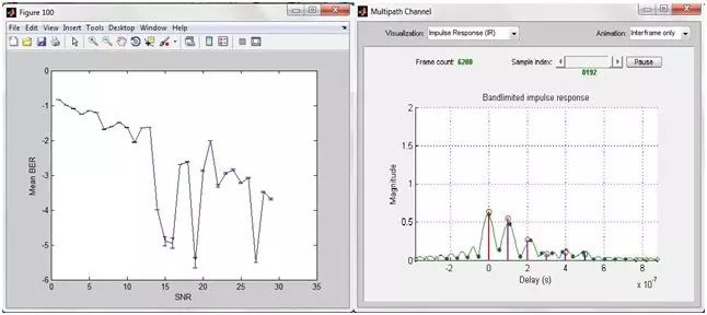
Results of these experiments are shown in figure 6.1, 6.2 and 6.3 respectively. Table 6.1, 6.2 and 6.3 gives the values of BER and average BER for all the values of SNR. If these three graphs are closely examined then it can be shown that the band limited impulse response increases as the speed increase and so as the BER and SNR.
The reason for such behavior is that because as the speed of the mobile increase, signal distortion also increases and it becomes difficult for the receiver to catch the signal, that’s the main reason that user travelling in high speed vehicle faces more distortion as compared to a pedestrian.
| SNR | BER & Average BER |
| SNR: 0 | BER:0.103833 |
| SNR: 0 | NoAvrg_BER:0.160358 |
| SNR: 5 | BER:0.014366 |
| SNR: 5 | NoAvrg_BER:0.033706 |
| SNR: 10 | BER:0.000206 |
| SNR: 10 | NoAvrg_BER:0.001528 |
| SNR: 15 | BER:0.000002 |
| SNR: 15 | NoAvrg_BER:0.000107 |
| SNR: 20 | BER:0.001543 |
| SNR: 20 | NoAvrg_BER:0.002319 |
| SNR: 25 | BER:0.000076 |
| SNR: 25 | NoAvrg_BER:0.000184 |
| SNR: 30 | BER:0.000000 |
| SNR: 30 | NoAvrg_BER:0.000164 |
BER & Average BER Vs. SNR for experiment 1
| SNR | BER & Average BER |
| SNR: 0 | BER:0.140855 |
| SNR: 0 | NoAvrg_BER:0.195596 |
| SNR:5 | BER:0.046527 |
| SNR:5 | NoAvrg_BER:0.071364 |
| SNR:10 | BER:0.011363 |
| SNR:10 | NoAvrg_BER:0.019860 |
| SNR:15 | BER:0.003815 |
| SNR:15 | NoAvrg_BER:0.006448 |
| SNR:20 | BER:0.000604 |
| SNR:20 | NoAvrg_BER:0.001222 |
| SNR:25 | BER:0.000214 |
| SNR:25 | NoAvrg_BER:0.000404 |
| SNR:30 | BER:0.000233 |
| SNR:30 | NoAvrg_BER:0.000503 |
| SNR | BER & Average BER |
| SNR: 0 | BER:0.128177 |
| SNR: 0 | NoAvrg_BER:0.182924 |
| SNR:5 | BER:0.056198 |
| SNR:5 | NoAvrg_BER:0.084254 |
| SNR:10 | BER:0.023229 |
| SNR:10 | NoAvrg_BER:0.035131 |
| SNR:15 | BER:0.006793 |
| SNR:15 | NoAvrg_BER:0.010362 |
| SNR:20 | BER:0.001748 |
| SNR:20 | NoAvrg_BER:0.002801 |
| SNR:25 | BER:0.000425 |
| SNR:25 | NoAvrg_BER:0.000691 |
| SNR:30 | BER:0.000354 |
| SNR:30 | NoAvrg_BER:0.000515 |
BER & Average BER vs. SNR for experiment 3
Although the results given by these simulations were quite accurate but they were not accurate enough to be trusted, as they were performing the process just for one period and getting the results on the basis of that.
Final MATLAB Model after Modifications
The initial MATLAB model is modified in this thesis, in order to use the same output from the channel model with different transmitter configurations to obtain more consistent results that can be compared with each other. Then theDVB-T2model will be modified so that it can be simulated using Matlab n times collecting data so that an x% confidence interval can be measured.
The results obtained after modifications were very consistent as they were performing the whole scenario for N times (defined by the user), this attribute lacks in the initial model as it was performing the complete task just for one cycle of time and any kind of distortion could fluctuate the results. While in modified model, the same process was performed by N times defined by the user and the results obtained are actually the average of all the cycles and hence providing a very consistent output, which couldn’t be distorted by any external factors.
Moreover, this new model further enhanced the initial model to calculate the Mean BER as it will give the overall performance of BER and average BER. Furthermore, calculates the standard BER on the basis of which global BER is also calculated.As the simulation of DVB-T2 requires a lot of input parameters from the user, that’s why a GUI is also designed in MATLAB, which makes the working of this project user friendly. User can easily change the parameters of the system using that GUI. On startup, the GUI looks like as shown in figure 4.2:
As mentioned above, taking all the other parameters constant, three experiments are performed for the mobile user moving at different speeds with different Iterations and no. of repeats, which are:
- Pedestrian moving at the speed of 0.1 km/h, with no of iterations = 500 and N=2.
- Bus moving at the speed of 5km/h, with no of iterations = 200 and N=2.
- Car moving at the speed of 10 km/h, with no of iterations = 1000 and N=2.
1.2.1 Results of First Experiment of Modified Model:
Results of the first experiment are shown in the figure 6.5, 6.6 and 6.7 respectively. While the theoretical values of BER and average BER for the corresponding SNR are shown in table 6.4 and the Mean BER and std BER are shown in table 6.5.
- Value of Global BER for the experiment comes out to be -2.4021.
| For N=1 | For N=2 | ||
| SNR: 0 | BER:0.131272 | SNR: 0 | BER:0.131542 |
| SNR: 0 | NoAvrg_BER:0.185916 | SNR: 0 | NoAvrg_BER:0.186218 |
| SNR:1 | BER:0.107086 | SNR:1 | BER:0.106672 |
| SNR:1 | NoAvrg_BER:0.157698 | SNR:1 | NoAvrg_BER:0.157319 |
| SNR:2 | BER:0.086805 | SNR:2 | BER:0.086459 |
| SNR:2 | NoAvrg_BER:0.129841 | SNR:2 | NoAvrg_BER:0.129562 |
| SNR:3 | BER:0.087178 | SNR:3 | BER:0.086924 |
| SNR:3 | NoAvrg_BER:0.128066 | SNR:3 | NoAvrg_BER:0.127755 |
| SNR:4 | BER:0.081465 | SNR:4 | BER:0.081709 |
| SNR:4 | NoAvrg_BER:0.116619 | SNR:4 | NoAvrg_BER:0.116581 |
| SNR:5 | BER:0.028071 | SNR:5 | BER:0.028074 |
| SNR:5 | NoAvrg_BER:0.051596 | SNR:5 | NoAvrg_BER:0.051751 |
| SNR:6 | BER:0.016450 | SNR:6 | BER:0.016439 |
| SNR:6 | NoAvrg_BER:0.030762 | SNR:6 | NoAvrg_BER:0.030725 |
| SNR:7 | BER:0.012705 | SNR:7 | BER:0.012607 |
| SNR:7 | NoAvrg_BER:0.022399 | SNR:7 | NoAvrg_BER:0.022108 |
| SNR:8 | BER:0.036446 | SNR:8 | BER:0.036612 |
| SNR:8 | NoAvrg_BER:0.052421 | SNR:8 | NoAvrg_BER:0.052642 |
| SNR:9 | BER:0.026200 | SNR:9 | BER:0.026378 |
| SNR:9 | NoAvrg_BER:0.039987 | SNR:9 | NoAvrg_BER:0.040434 |
| SNR:10 | BER:0.014162 | SNR:10 | BER:0.014155 |
| SNR:10 | NoAvrg_BER:0.023779 | SNR:10 | NoAvrg_BER:0.023805 |
| SNR:11 | BER:0.007526 | SNR:11 | BER:0.007539 |
| SNR:11 | NoAvrg_BER:0.013874 | SNR:11 | NoAvrg_BER:0.013838 |
| SNR:12 | BER:0.015524 | SNR:12 | BER:0.015382 |
| SNR:12 | NoAvrg_BER:0.023693 | SNR:12 | NoAvrg_BER:0.023602 |
| SNR:13 | BER:0.005303 | SNR:13 | BER:0.005448 |
| SNR:13 | NoAvrg_BER:0.008758 | SNR:13 | NoAvrg_BER:0.008764 |
| SNR:14 | BER:0.008712 | SNR:14 | BER:0.008823 |
| SNR:14 | NoAvrg_BER:0.014517 | SNR:14 | NoAvrg_BER:0.014421 |
| SNR:15 | BER:0.013224 | SNR:15 | BER:0.013144 |
| SNR:15 | NoAvrg_BER:0.019547 | SNR:15 | NoAvrg_BER:0.019305 |
| SNR:16 | BER:0.001919 | SNR:16 | BER:0.001890 |
| SNR:16 | NoAvrg_BER:0.003767 | SNR:16 | NoAvrg_BER:0.003703 |
| SNR:17 | BER:0.002873 | SNR:17 | BER:0.002907 |
| SNR:17 | NoAvrg_BER:0.004932 | SNR:17 | NoAvrg_BER:0.005001 |
| SNR:18 | BER:0.000610 | SNR:18 | BER:0.000641 |
| SNR:18 | NoAvrg_BER:0.001197 | SNR:18 | NoAvrg_BER:0.001243 |
| SNR:19 | BER:0.006294 | SNR:19 | BER:0.006231 |
| SNR:19 | NoAvrg_BER:0.009262 | SNR:19 | NoAvrg_BER:0.009209 |
| SNR:20 | BER:0.001799 | SNR:20 | BER:0.001749 |
| SNR:20 | NoAvrg_BER:0.003268 | SNR:20 | NoAvrg_BER:0.003248 |
| SNR:21 | BER:0.000966 | SNR:21 | BER:0.000998 |
| SNR:21 | NoAvrg_BER:0.001677 | SNR:21 | NoAvrg_BER:0.001636 |
| SNR:22 | BER:0.001733 | SNR:22 | BER:0.001778 |
| SNR:22 | NoAvrg_BER:0.002772 | SNR:22 | NoAvrg_BER:0.002883 |
| SNR:23 | BER:0.004920 | SNR:23 | BER:0.004914 |
| SNR:23 | NoAvrg_BER:0.007638 | SNR:23 | NoAvrg_BER:0.007743 |
| SNR:24 | BER:0.000089 | SNR:24 | BER:0.000098 |
| SNR:24 | NoAvrg_BER:0.000220 | SNR:24 | NoAvrg_BER:0.000234 |
| SNR:25 | BER:0.000001 | SNR:25 | BER:0.000001 |
| SNR:25 | NoAvrg_BER:0.000052 | SNR:25 | NoAvrg_BER:0.000052 |
| SNR:26 | BER:0.000408 | SNR:26 | BER:0.000393 |
| SNR:26 | NoAvrg_BER:0.000695 | SNR:26 | NoAvrg_BER:0.000646 |
| SNR:27 | BER:0.000583 | SNR:27 | BER:0.000600 |
| SNR:27 | NoAvrg_BER:0.001222 | SNR:27 | NoAvrg_BER:0.001242 |
| SNR:28 | BER:0.000352 | SNR:28 | BER:0.000381 |
| SNR:28 | NoAvrg_BER:0.000609 | SNR:28 | NoAvrg_BER:0.000625 |
| SNR:29 | BER:0.000107 | SNR:29 | BER:0.000124 |
| SNR:29 | NoAvrg_BER:0.000365 | SNR:29 | NoAvrg_BER:0.000384 |
| SNR:30 | BER:0.000367 | SNR:30 | BER:0.000351 |
| SNR:30 | NoAvrg_BER:0.000720 | SNR:30 | NoAvrg_BER:0.000695 |
SNR Vs. BER values for Experiment 1
| Mean BER | std BER |
| -0.8814 | 0.0006 |
| -0.9711 | 0.0012 |
| -1.0623 | 0.0012 |
| -1.0602 | 0.0009 |
| -1.0884 | 0.0009 |
| -1.5517 | 0.0000 |
| -1.7840 | 0.0002 |
| -1.8977 | 0.0024 |
| -1.4374 | 0.0014 |
| -1.5802 | 0.0021 |
| -1.8490 | 0.0001 |
| -2.1231 | 0.0005 |
| -1.8110 | 0.0028 |
| -2.2696 | 0.0083 |
| -2.0571 | 0.0039 |
| -1.8799 | 0.0019 |
| -2.7203 | 0.0046 |
| -2.5391 | 0.0035 |
| -3.2039 | 0.0151 |
| -2.2033 | 0.0031 |
| -2.7511 | 0.0086 |
| -3.0078 | 0.0099 |
| -2.7556 | 0.0079 |
| -2.3083 | 0.0004 |
| -4.0308 | 0.0285 |
| -6.1938 | 0 |
| -3.3978 | 0.0118 |
| -3.2281 | 0.0086 |
| -3.4365 | 0.0247 |
| -3.9387 | 0.0460 |
| -3.4455 | 0.0137 |
Mean BER & std BER values for Experiment 1
1.2.2 Results of Second Experiment of Modified Model:
Figure 6.8, 6.9 and 6.10 gives us the results for the experiment 2, when user is travelling at the speed of 1km/s and the no of iterations taken here are 500 with repeat cycle i.e. N=2. Table 6.6 and 6.7 gives us the values of SNR vs. BER and the Mean BER and standard BER respectively.- Global BER comes out for experiment 2 was –inf.
| For N = 1 | For N = 2 | ||
| SNR: 0 | BER:0.144963 | SNR: 0 | BER:0.144537 |
| SNR: 0 | NoAvrg_BER:0.200382 | SNR: 0 | NoAvrg_BER:0.200617 |
| SNR:1 | BER:0.103536 | SNR:1 | BER:0.103496 |
| SNR:1 | NoAvrg_BER:0.153318 | SNR:1 | NoAvrg_BER:0.153312 |
| SNR:2 | BER:0.081079 | SNR:2 | BER:0.081874 |
| SNR:2 | NoAvrg_BER:0.123080 | SNR:2 | NoAvrg_BER:0.123966 |
| SNR:3 | BER:0.056279 | SNR:3 | BER:0.056618 |
| SNR:3 | NoAvrg_BER:0.096223 | SNR:3 | NoAvrg_BER:0.096636 |
| SNR:4 | BER:0.070647 | SNR:4 | BER:0.070241 |
| SNR:4 | NoAvrg_BER:0.103436 | SNR:4 | NoAvrg_BER:0.103023 |
| SNR:5 | BER:0.063094 | SNR:5 | BER:0.063427 |
| SNR:5 | NoAvrg_BER:0.089725 | SNR:5 | NoAvrg_BER:0.090577 |
| SNR:6 | BER:0.020785 | SNR:6 | BER:0.021318 |
| SNR:6 | NoAvrg_BER:0.039970 | SNR:6 | NoAvrg_BER:0.040469 |
| SNR:7 | BER:0.024660 | SNR:7 | BER:0.024455 |
| SNR:7 | NoAvrg_BER:0.040979 | SNR:7 | NoAvrg_BER:0.041170 |
| SNR:8 | BER:0.032986 | SNR:8 | BER:0.032662 |
| SNR:8 | NoAvrg_BER:0.052140 | SNR:8 | NoAvrg_BER:0.052100 |
| SNR:9 | BER:0.023306 | SNR:9 | BER:0.022988 |
| SNR:9 | NoAvrg_BER:0.037168 | SNR:9 | NoAvrg_BER:0.037283 |
| SNR:10 | BER:0.009120 | SNR:10 | BER:0.008878 |
| SNR:10 | NoAvrg_BER:0.017749 | SNR:10 | NoAvrg_BER:0.017499 |
| SNR:11 | BER:0.023258 | SNR:11 | BER:0.023224 |
| SNR:11 | NoAvrg_BER:0.034964 | SNR:11 | NoAvrg_BER:0.034473 |
| SNR:12 | BER:0.023534 | SNR:12 | BER:0.023745 |
| SNR:12 | NoAvrg_BER:0.034579 | SNR:12 | NoAvrg_BER:0.034325 |
| SNR:13 | BER:0.000103 | SNR:13 | BER:0.000101 |
| SNR:13 | NoAvrg_BER:0.000588 | SNR:13 | NoAvrg_BER:0.000648 |
| SNR:14 | BER:0.000016 | SNR:14 | BER:0.000010 |
| SNR:14 | NoAvrg_BER:0.000196 | SNR:14 | NoAvrg_BER:0.000231 |
| SNR:15 | BER:0.000009 | SNR:15 | BER:0.000014 |
| SNR:15 | NoAvrg_BER:0.000209 | SNR:15 | NoAvrg_BER:0.000240 |
| SNR:16 | BER:0.001996 | SNR:16 | BER:0.002008 |
| SNR:16 | NoAvrg_BER:0.003367 | SNR:16 | NoAvrg_BER:0.003535 |
| SNR:17 | BER:0.002367 | SNR:17 | BER:0.002430 |
| SNR:17 | NoAvrg_BER:0.003467 | SNR:17 | NoAvrg_BER:0.003535 |
| SNR:18 | BER:0.000002 | SNR:18 | BER:0.000004 |
| SNR:18 | NoAvrg_BER:0.000010 | SNR:18 | NoAvrg_BER:0.000018 |
| SNR:19 | BER:0.001298 | SNR:19 | BER:0.001367 |
| SNR:19 | NoAvrg_BER:0.002071 | SNR:19 | NoAvrg_BER:0.002116 |
| SNR:20 | BER:0.009918 | SNR:20 | BER:0.009850 |
| SNR:20 | NoAvrg_BER:0.014701 | SNR:20 | NoAvrg_BER:0.014585 |
| SNR:21 | BER:0.000472 | SNR:21 | BER:0.000521 |
| SNR:21 | NoAvrg_BER:0.000769 | SNR:21 | NoAvrg_BER:0.000854 |
| SNR:22 | BER:0.001085 | SNR:22 | BER:0.001169 |
| SNR:22 | NoAvrg_BER:0.001855 | SNR:22 | NoAvrg_BER:0.001917 |
| SNR:23 | BER:0.001360 | SNR:23 | BER:0.001495 |
| SNR:23 | NoAvrg_BER:0.002240 | SNR:23 | NoAvrg_BER:0.002427 |
| SNR:24 | BER:0.000595 | SNR:24 | BER:0.000621 |
| SNR:24 | NoAvrg_BER:0.001258 | SNR:24 | NoAvrg_BER:0.001321 |
| SNR:25 | BER:0.000873 | SNR:25 | BER:0.000820 |
| SNR:25 | NoAvrg_BER:0.001457 | SNR:25 | NoAvrg_BER:0.001422 |
| SNR:26 | BER:0.000003 | SNR:26 | BER:0.000003 |
| SNR:26 | NoAvrg_BER:0.000199 | SNR:26 | NoAvrg_BER:0.000201 |
| SNR:27 | BER:0.000326 | SNR:27 | BER:0.000342 |
| SNR:27 | NoAvrg_BER:0.000637 | SNR:27 | NoAvrg_BER:0.000651 |
| SNR:28 | BER:0.000198 | SNR:28 | BER:0.000216 |
| SNR:28 | NoAvrg_BER:0.000270 | SNR:28 | NoAvrg_BER:0.000262 |
| SNR:29 | BER:0.000000 | SNR:29 | BER:0.000000 |
| SNR:29 | NoAvrg_BER:0.000000 | SNR:29 | NoAvrg_BER:0.000000 |
| SNR:30 | BER:0.000000 | SNR:30 | BER:0.000000 |
| SNR:30 | NoAvrg_BER:0.000071 | SNR:30 | NoAvrg_BER:0.000078 |
SNR Vs. BER values for Experiment 2
| Mean BER | Std BER |
| 0.8394 | 0.0009 |
| 0.9850 | 0.0001 |
| 1.0890 | 0.0030 |
| 1.2483 | 0.0018 |
| 1.1522 | 0.0018 |
| 1.1989 | 0.0016 |
| 1.6767 | 0.0078 |
| 1.6098 | 0.0026 |
| 1.4838 | 0.0030 |
| 1.6355 | 0.0042 |
| 2.0458 | 0.0083 |
| 1.6337 | 0.0005 |
| 1.6264 | 0.0027 |
| 3.9915 | 0.0072 |
| 4.8895 | 0.1323 |
| 4.9486 | 0.1512 |
| 2.6985 | 0.0018 |
| 2.6201 | 0.0081 |
| 5.5089 | 0.1569 |
| 2.8755 | 0.0159 |
| 2.0051 | 0.0021 |
| 3.3048 | 0.0302 |
| 2.9484 | 0.0231 |
| 2.8460 | 0.0291 |
| 3.2160 | 0.0133 |
| 3.0727 | 0.0192 |
| 5.4949 | 0 |
| 3.4765 | 0.0154 |
| 3.6850 | 0.0273 |
| Inf | NaN |
| Inf | NaN |
Mean BER and std BER values for Experiment 2
Remarks
This thesis presents the design and Implementation of DVB-T2 system in MATLAB software. The basic purpose of this thesis is to check the bit error ratio (BER) and signal to noise ratio (SNR) for DVB-T2 system so that the system could be improved to a better quality. DVB-T2 system is evaluated for mobile users moving at different speeds. It is clearly shown that the mobility has an impact on the received signal, where the SNR goes to zero in some points. This behavior will generate high BER. If the figures for impulse responses are checked for all the three experiments then it is depicted that the Impulse is high for the third experiment where the mobility speed is higher than the first two experiments. The packet data loss is almost zero for the first experiment while it’s increasing in the second and is higher in the third. The number of packet lost confirms this behavior that high losses occurred in the case of high mobility.
