Sensorless Speed Estimation of Induction Motor in MATLAB

Today I am going to show you Sensorless Speed Estimation of Induction Motor in MATLAB. In order to control and estimate the speed of Induction motor, there are many methods proposed by different scientists. The method I have selected in my project is Adaptive method. Using this method, I have controlled the speed of Induction motor using MATLAB software. Matlab software is used for simulation design. The simulation is designed in simulink and the MATLAB version used for designing this project is MATLAB 2010. It is also tested on MATLAB 2012 and 2013. All the details of this project are mentioned below.

If someone wants to buy this project then click on the button shown on right side. Its quite difficult to implement and is designed because of the efforts of our team that's why we haven't made it open source but we have placed a very small purchase amount because mostly it is asekBefore going into the details of Induction motor, let’s first have a look on the mathematical derivations. Few of the well-known methods are:

1. Adaptive Method.
2. Least-Squares Method.
3. Non Linear Method.

Mathematical Derivation - Sensorless Speed Estimation of Induction Motor

In order to apply the adaptive method on the Induction motor, there was a need to first design the induction motor on Simulink. For designing the Induction motor on Simulink, mathematical calculations were required. So, my first task was to derive the complete mathematical equations for all the variables of Induction motor.

The basic mathematical model also known as the a-b model (or two-phase equivalent model) of induction motor is given as:

• ? is the rotor angular velocity.
• ?_Ra& ?_Rb are the rotor magnetic fluxes.
• i_Sa and i_Sbare the stator currents.
• s = 1 – M­­­²/ L_R L_Salso known as leakage parameter.

Adaptive Method Calculation

The approach used in this report is to consider the speed as an unknown constant parameter. The reason for choosing this parameter is that it changes slowly as compared to all the other electrical parameters and as it changes slowly so it can be controlled more effectively. The adaptive method techniques are applied on the speed parameter and thus estimated it. This adaptive method approach on speed parameter was first implemented by Shauder and are further enhanced and researched by Peng and Fukao. Using the last two equations of the system (1), I derived the below equations:

• ?_maand ?_mb are the magnetic fluxes and are thus known quantities.

Now take the second and third equations of system (1) and divide them by M / L_R and then differentiate them w.r.t time and the below equations are obtained:

• d? / dt = 0 as we have already assumed in this approach that the speed will remain constant.

System (3) gives us the derivative of magnetic fluxes. In order to calculate the error dynamics induced in the system, we need to calculate the estimated values of these magnetic fluxes and then subtract them from the system (3). The estimated values of the magnetic fluxes are as follows:

V (e_ma, e_mb) = ½ (e²_ma + e²_mb)

Using the above equation and the values of e_ma and e_mb, we get:

Modeling in Simulink

The model designed in MATLAB is shown in the figure 1. This model is performing the simulation of motor moving in both the directions i.e. clockwise and anti-clockwise. It contains four main blocks, which are:

• 3-Phase Input Voltage with variable Frequency.
• V_abcto stationary frame conversion block.
• Motor system block.
• Speed estimation block.

All these four blocks are discussed below in detail:

3-Phase Input Voltage with variable Frequency

This block, as the name depicts, is used for generating variable frequencies. In the start, the first model, I generated, was for fixed frequency of induction motor and was also showing just one direction of motor. So, I did few modifications in the model and added this block so that the motor could move both in positive and negative directions and can also move at different frequencies.

Figure 2 shows the parameter block for this block and from this block one can set the frequency of this motor quite easily. From this parameter block, one can set:

• Amplitude of the input signals.
• Phase difference between the input signals.
• Frequencies of these input signals.

By default, I have taken two frequencies, for which the motor will rotate during a cycle.

Reverse Direction of motor

In order to change the direction of the motor, I have used the phase change. When the voltage applied to the motor reverses its direction, the direction of the motor also reverses. For this simulation, the motor will rotate in clockwise direction when:

• Phase of Va = 0
• Phase of Vb = -2*pi/3
• Phase of Vc = -4*pi/3

And it will reverse the direction, when:

• Phase of Va = 0
• Phase of Vb = -4*pi/3
• Phase of Vc = -2*pi/3

i.e. Vb and Vc are changing their positions. In order to do so I added a phase change in this block and thus for the first 5 sec the motor will move in one direction and for the last 5 sec it will move in the opposite direction automatically.

V_abcto Stationary Frame Conversion Block:

This block is separately shown in the figure 2. This block takes V_abc as an input and gives output in the form of V(alpha) and V(beta). This conversion is known as Clarke Transformation. This transformation is used in order to simplify the implementation of three phase systems as in Clarke Transformation, a reference signal is obtained. V (gamma) becomes zero in Clarke Transformation that’s why it becomes very easy to use.

In Clarke Transformation, the relation between V_abc and V (alpha) and V (beta) is given as:

If we closely examine the figure 3, then it is shown that inputs coming are V_a, V_b and V_c. After that the above equations are applied on these input signals and the output received is V (alpha) and V (beta). In simple words, figure 3 is implementation of Clarke Transformation.

• V_a, V_b and V_c are simple sine waves with amplitude of 2300 and frequency of 50 rad/s.
• As it’s a three phase system so all these three signals have a phase difference of 120^o.

• V (alpha) and V (beta) obtained after the Clarke Implementation are shown in the Figure 4.

Motor System Block:

Motor system block is the practical implementation of set of equations shown in the system (1). It is the basic mathematical model of Induction motor shown in figure 5. It is taking V (alpha) and V (beta) as an input along with the load applied on Induction motor. In other words, I can say that this block is the actual Induction motor and I need to apply the adaptive method technique on this block in order to estimate and control its speed.

V (alpha) and V (beta) applied here are the same obtained in the Clarke Transformation explained in the previous section. Outputs of this function are the states which we will study in detail in the fourth section and the derivatives of currents I_sa and I_sb.

Let’s double click this motor system block and check the functions it’s calculating. The functions of this sub system are shown in the figure 6. As I told earlier, this block is the simulation of system (1), which is also shown below:

As shown in the figure 6, motor block is implementing all the five equations of system (1), which are:

• First block in Figure 6 is calculating d?_Ra/dtwhich is the equation 2 of the system 1.
• Second block in Figure 6 is calculating d?_Rb/dtwhich is the equation 3 of the system 1.
• Third block in Figure 6 is calculating d? /dtwhich is the equation 1 of the system 1.
• Fourth block in Figure 6 is calculating u_sawhich is the equation 4 of the system 1.
• Fifth block in Figure 6 is calculating u_sbwhich is the equation 5 of the system 1.

All these functions are shown in the figures 7(a-e).

Figure 7c: Implementation of equation 1 of system 1

Figure 7d: Implementation of equation 4 of system 1

Figure 7e: Implementation of equation 5 of system 1

• Graphical representation of all these systems are shown in the figure 7(f, g, h, i).

Figure 7f: Graphical Representation of equation 2 of system 1

Figure 7g: Graphical Representation of equation 3 of system 1

Figure 7h: Graphical Representation of equation 4 of system 1

Figure 7i: Graphical Representation of equation 5 of system 1

After the implementation of all these equations, a complete model of Induction motor has been obtained. Now there’s a need to apply the technique of adaptive method on it so that the speed could be controlled without the help of sensor, which is done explained in detail in the next section.

In order to change the parameter of this system, I have added a parameter block in it shown in the below figure:

Speed Estimation Block:

Let's have a look at the Speed Estimation Block of Sensorless Speed Estimation of Induction Motor in MATLAB. Speed Estimation is the place where adaptive method technique is applied to estimate the speed of Induction motor. This block is actually implementing the system (3) and system (4) and thus calculating the real speed and the estimated speed of the Induction motor respectively. After the calculation of these speeds, it is further calculating the error dynamics by subtracting the estimated speed from the real speed.

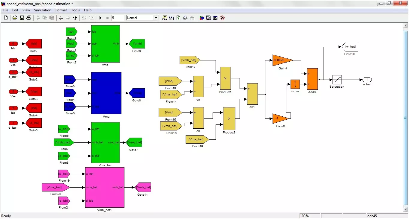
Speed Estimation block is shown in the figure 8. Inputs coming to the speed estimation are the same obtained in the first and second block i.e. V (alpha), V (beta), I_sa, I_sb, dI_sa/dt and dI_sb/dt. The functions implemented by this subsystem are shown in the figure 9.

Figure 9: Functions Implemented by System Estimation Block

System (3) and system (4) are implemented in the figure 9, which are as follows:

• First green block in the figure 9 is implementing the equation 2 of the system 3.
• Second blue block in the figure 9 is implementing equation 1 of the system 3.

Thus the outputs of these two blocks will give us the real speed values.

• Third green block in the figure 9 is implementing the equation 2 of the system 4.
• Fourth pink block of the figure 9 is implementing the equation 1 of the system 4.

So, the output of these two blocks will give us the value of estimated speed. The internal functions of all these four blocks are shown in figures 10a, 10b, 10c and 10d respectively.

Figure 10a: Implementation of Equation 2 of System 3.

Figure 10b: Implementation of Equation 1 of System 3.

Figure 10c: Implementation of Equation 2 of System 4.

Figure 10d: Implementation of Equation 1 of System 4.

After the calculation of all the four values, the speed estimator block then implemented the system (5), which is:

Implementation of this system 5 is separately shown in the figure 11, which finally gives us the value of estimated speed.

Graph of both the estimated speed and the actual speed is shown in the figure 12.

Figure 12: Graph of Estimated Speed and Actual Speed

Conclusion:

Let's have a look at the conclusion of Sensorless Speed Estimation of Induction Motor in MATLAB. Figure 12 shows both the actual and estimated speed induction motor. In the start, the motor is moving at the speed of around 25 rpm, after that the speed is increased to 50 rpm, and the motor starts to rotate in the opposite direction that’s why the graph shows the negative value. Now, it’s moving at 50 rpm in the opposite direction and lastly, it is moving at 25 rpm in the opposite direction. Figure 13 shows the graph for estimated errors. It is quite obvious from the error graph that whenever the speed of the motor fluctuates the error goes quite high. In other words, the acceleration produced in the motor causes the error to increase while the error remains zero when the motor is moving at constant speed, regardless of direction.

Figure 13: Estimated Error Dynamics