Special Matrix Commands in MATLAB


Hello learners. Welcome to The Engineering Projects. We all know that matrices have been used in the engineering field for a long time, and they have a vital role in the calculation of different data. Therefore, we are learning about some very special kinds of matrices that are usually introduced to engineers at a higher level. Till now, we have seen some general operations on matrices and also examined the special kinds of matrices. Yet, today, we are moving a step forward and learning about some complex types of matrices that require strong basic concepts. So, have a glimpse at the topics that you are going to learn, and then, we’ll start practicing.
What is a matrix?
What are the different types of matrices that are less common?
How can we implement some interesting commands in MATLAB?
What is the procedure for dealing with complex equations in MATLAB?
What is a Matrix?
First of all, it is recommended to learn about the introduction of the matrix. A matrix has different elements in it with different sequences, and we define it as:
“A matrix is a rectangular array in which different types of elements in the different sequences are present, and all the elements are enclosed in a long bracket that is usually a square bracket.”
The sequence and the values of the matrices are important, and the collection of horizontal lines is called a row. On the other hand, the vertical entries are collectively called columns. To find the difference in the types of matrices, it is important to know that the basic kinds of matrices are square matrix and rectangular matrix. Most of the matrices that we are going to discuss here will be square matrices.
Types of Matrices
Depending upon different parameters in matrices, these are divided into different types and groups. In a square matrix, the numbers of rows and columns are equal to each other, and in a rectangular matrix, the numbers of rows and columns are never equal. You will observe different parameters on the basis of which these matrices are recognized, and then the behavior of each of them is examined. So have a look at these types.
A Boolean Matrix
We all know that boolean numbers mean two conditions only, that are, zero and one. So, the boolean matrix is the type of matrix in which only zero and one value are used, and other values are never involved. The order of the matrix may be anything, but the entries must be either zero or one.

One thing that must be kept in mind is that the matrix will surely have these values in a non-specific pattern and it never has only zero or only one. There must be one and zero of each type. We are clearing it because some other types, such as singular matrix, identity matrix, null matrix, and scalar matrix, also involve zero and one, but in a specific manner.
Boolean numbers and conditions are used in almost every field of mathematics, and therefore, this matrix is also used in different ways in such fields. With the help of a matrix, it becomes easy to deal with a large number of data points at once. The example we have shown here has a small size. Yet, when the boolean matrix is used in practical life, we use a bulk of matrices with greater sizes.
Orthogonal Matrices
In the previous section, we learned that a transpose of the matrix is obtained when the rows and columns, along with the entries, are interchanged with each other. Keeping this concept in mind, we can define this type of matrix as
A matrix A is called an orthogonal matrix if and only if the multiplication of the matrix A with the transpose of itself provides us with the identity matrix.
If you are new to the identity matrix, then you must know that an identity matrix is one that contains only value 1 in its diagonal and all the entries other than the diagonal are zero.
The inverse of a Matrix
As we have read about the orthogonal matrices, they remind us of the inverse of the matrix. It is interesting to know that there exists the inverse of a matrix that, when multiplied with the original matrix, delivers us the identity matrix. We hope you remember that an identity matrix is a type of matrix that always has the value 1 in the diagonal elements and zero in all the remaining elements. So, if we are taking matrix A, then for the inverse matrix, we can say:
A.AT= I
In this way, if we have the value of A and want to know the inverse of it, we use the following equation:
AT= I/A

So, in this way, we have observed that no matter if the inverse of the matrix is multiplied with the original matrix or vice versa, we get the identity matrix. This condition is somehow special because the multiplication of the matrix is a more complex operation than addition and subtraction, yet here we are using the rules of the dot product. There is another way to find the inverse of a matrix with the help of a formula that states that the inverse of a matrix A is equal to the determinant of matrix A with an adjoint of A.
There are certain conditions for the existence of a square matrix:
A matrix has the inverse only if it is a square matrix.
If the determinant of the matrix is equal to zero, then there is no need to find the adjoint of that matrix because the inverse does not exist for that matrix.
It is not always necessary that in the inverse of a matrix, the values are reciprocal of the original matrix. The values may also be changed, and by dot multiplication, we can get the identity matrix.
Stochastic Matrix
Here is another interesting type of matrix in which all the values show the probability values. We know that the probability values are so small that they are less than one and have fractional values or in the form of points less than one. So, the stochastic matrix has all the probability values as its elements.

You can see all the values are less than one because the probability is usually in the form of such small numbers. If any of the values is greater, then it is not a stochastic matrix.
Nilpotent Matrix
This is a less common type of matrix in which Ak = O, that is, for every power of the matrix, we get a null matrix (the one with all the values equal to zero). There are two conditions that must be fulfilled in this type:
The matrix A must be square.
We get a null matrix every time we apply any power to matrix A, which is a natural number.
For example, when we take the square of each value of A, we get the null matrix. It is a less common type of matrix, but at a higher level of calculations, it has its applications.
Idemportenet Matrix
It is a type of uncommon matrix that provides us with a matrix equal to itself when any power is applied to it greater than 2. That is, An = A where the value of n is always equal to or greater than 2. Usually, it has been noticed that if the square of the matrix A is equal to itself, then there is no need to check further because the result remains the same for any number greater than 2. You can take it as homework and find examples of such matrices by yourself.
Special Commands in MATLAB
It seems like you have learned a lot about the special kinds of matrices. When we talk about MATLAB, we have observed that there are different MATLAB commands that are not related directly to the matrices yet are used to make the functioning of a group of numbers and matrices easier and more effective in some cases. So, have a look at some of the commands.

sr# |
Command |
Description |
1 |
inv(A) |
This provides us with the inverse of the matrix A. |
2 |
s,t, complex(s,t) |
It is the way to introduce a complex number in MATLAB. It produces a complex equation with s as a real number and t as an imaginary number. |
3 |
real(A) |
With the help of this command, you can find the real part of the equation saved as equation A. |
4 |
imag(A) |
By using this command, you can easily encounter the real part of the equation saved as equation A. |
5 |
abs(A) |
This command will show us the absolute value of the matrix A. |
6 |
angle(A) |
To find the angle of equation A, we use this command. |
The procedure to perform the Complex Number in MATLAB
We all know about complex numbers and have also used them in the matrices when we were talking about hermitian metrics. A special kind of function in MATLAB is the “complex” function, which is used to make the complex equation. So have a look at the step-by-step procedure to perform the complex equation in MATLAB.
Hit the start button of MATLAB.
Go to the command window.
Start by writing the following command.
a=3
w=3
It will provide us with two numbers that we will use in the complex function. We are naming this equation ComplexEqaution, and the command to perform this is
ComplexEqaution=complex(a,w)
Press the enter button.
Now, using this equation, we can also find the real and imaginary parts of the equation using different commands. For real numbers, we are writing:
real(ComplexEqaution)
It will give us the real part of the equation. Similarly, write the following command for the imaginary number:
imag(ComplexEqaution)
Similarly, to obtain the absolute value of the equation we have just made, we are using the required command.
abs(ComplexEqaution)
Finally, to find the angle of the equation, we are using its command.
angle(ComplexEqaution)
Now, to perform the inverse of a matrix, we are going to introduce the matrix first. So, write the following command:
B=[1 55 2 7; 4 5 2 8; 4 99 1 6; 3 8 4 1]
The command for this purpose is:
InversofMatrix= inv(B)
If you are confused about the absolute value of the complex equation, then you must realize that complex numbers are present in the plane or the coordinates of the system, and the absolute value of the complex numbers is defined as the total distance between the origin of the complex number (where the plane is (0,0)) and the complex plane (a,b). The procedure to do so is a little bit complex if we solve it theoretically, but with the help of MATLAB, this can be done with the help of a simple command and all the control in your hand. You should practice more with all these commands by using your own values in the matrix with a different sequence. Once you have followed all the instructions given above, the output at your MATLAB command window should be like the images given next:


So, in this way, we have gotten rid of the long and error-prone calculations, and by using simple commands, we have simply applied the formula of inverse, and in this way, we have not had to find the adjoint and determinant of the matrix A.
Consequently, we had a little bit of a complex yet interesting lecture today on matrix, in which we defined it first for a solid foundation of the concept. After that, there were different types of matrices that are less common but have interesting patterns of the elements in which the values and positions are important to define the type of matrix. Moreover, we have seen some interesting commands in MATLAB to perform the operations of complex equations and also implement them all practically. In the next lecture, you are going to learn the amazing features and applications of MATLAB in different aspects of the study.