Fault Detection of Gas Turbine in MATLAB

Hello friends, I hope you all are fine and enjoying. Today i am going to share a new project which is Fault Detection of Gas Turbine in MATLAB. In this project, i will try to elaborate that, What is a Gas Turbine? What are the operating parameters of a Gas Turbine? Mostly what type of Faults and Vibrations comes in Gas Turbine system during its operation? Gas Turbine is also called a Combustion Turbine. It has Four Basic components which includes Compressor, Combustion Chamber, Turbine and Alternator.
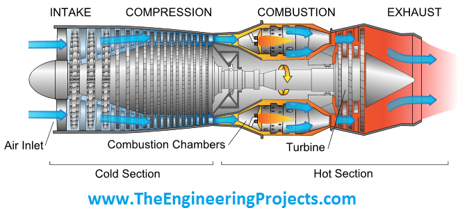
Generally compressor is installed upstream and the Rotating turbine is connected downstream and the Combustion Chamber is connected in between both of them and at the end of line we have Alternator which is also connected on the same shaft.Gas Turbine operates on "Brayton Cycle". Gas Turbine can be divided into 2 main sections, COLD Section and HOT Section, as shown in the above feature image. COLD Section includes Compressor and the HOT Section includes Turbine and and Exhaust portion. First of all, Compressor in-takes the Fresh atmospheric air and after compression it gets to high pressure, next comes the Combustion Chamber in which fuel is sprayed continuously and ignites the air so that combustion generates a High-Temperature Flow. In the next stage, this high temperature and high pressure gas enters into turbine and it releases its energy to turbine blades and the Turbine starts to rotate. A synchronous generator is also connected on the same shaft of the Turbine and when turbine gets to its rated rpm, then synchronous generator starts to generate electricity. Gas Turbines are of different Sizes and Ratings. The operation of Gas Turbine includes to monitor a large no of parameters. For example During the operation of Gas Turbine, a large no. of equipments are operating simultaneously and there are always chances of some fault occurrence and some abnormal vibrations. Although we also have a large no of primary and secondary protection equipments installed but we still need very careful monitoring of the system for its safe operation. Gas turbines are widely used in aircraft engines, trains, ships and coupled with electrical generators to generate electricity.
It was quite a tough job of design the Model of Gas Turbine in Simulink and it includes a lot of our team efforts, so we haven't made it a open source and we have placed a very small amount for this which is, 10$ only. You can click on the above button to purchase the complete control model of Gas Turbine in Simulink. Above was a small introduction about the basic components of Gas Turbine and their operation. Now lets move towards the designing of the Fault Detection of Gas Turbine in MATLAB.
You may also like to read:
Fault Detection of Gas Turbine in MATLAB
- In order to observe the Fault Detection of Gas Turbine in MATLAB, we are gonna use Simulink which is available in MATLAB.
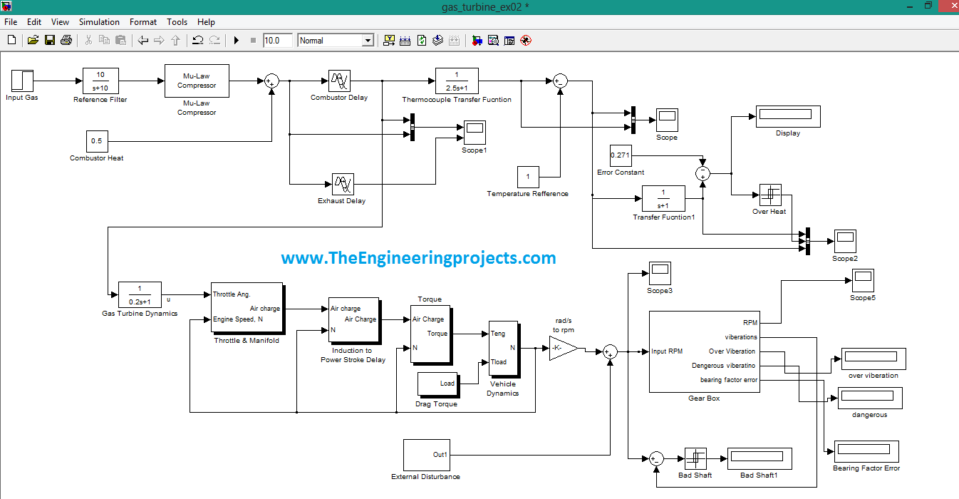
- The complete Simulink model of Gas Turbine is shown in the image given below:
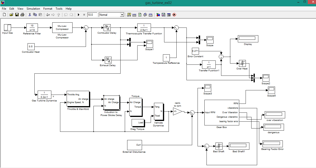
- First of all fresh air from atmosphere is entered into the system and and next to that we have a 'Reference Filter', which removes dust particles from air.
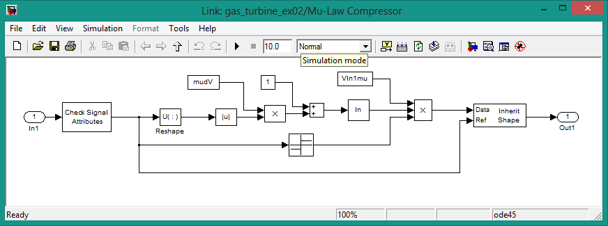
- Next to that, we have a Mu- Law compressor and to see the other properties of this compressor you will select that icon and then right click on it, a window will open and then you will click on option 'look under mask' .
- When you will click that option, a new window will open in Simulink and it will be representing the actual parameters of Mu-Law compressor.
- You can see that in the figure given below:
- The output of Mu-Law compressor comes to a summing junction and at this junction, we also have another input which is of Combustor Heat.
- The output of the summing junction goes to the combustor delay and exhaust delay.
- The output of combustor delay and the exhaust delay is connected to a scope.
- The purpose of scope is to see the actual output graphical parameters of the of the combustion delay and exhaust delay and we can also check some abnormalities through it.
- The output of combustor relay goes to Gas Turbine Dynamics. It is Gas Turbine built in function and it is used to observe the dynamic behavior of Gas Turbine. The Gas Turbines Dynamics control are shown in the image below:
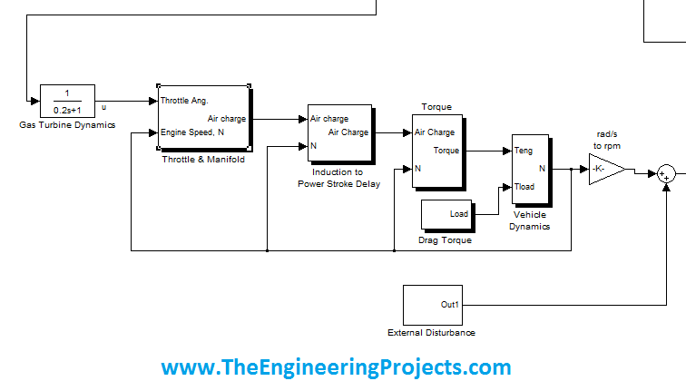
- The output of Gas Turbine goes to 'Throttle and Manifold' control. This control is observing the air intake dynamics of the gas turbine.
- If you double click on it, then a new window will open which will be showing the embedded close loop system of 'Throttle and Manifold ' control, which can be easily seen in the image given below:
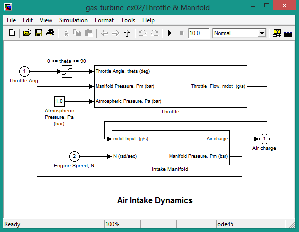
- First comes the throttle angle control of gas turbine. It has three inputs.
- First input is the Throttle angle 'Theta' and this angle is measured in 'degrees'.
- Second input is of the atmospheric pressure which is measured in 'bar', as you can see in the above image.
- Third input is of the 'Manifold Pressure' and it is also measured in bar.
- Manifold is actually the output of second control system which is also embedded in the same system.
- From above image, we see that on the next stage, output of 'Throttle Control' is actually the the input of 'Manifold Control' system and second input of manifold system is Engine Speed which is actually the speed of Gas Turbine and it is measured in rad/sec.
- The whole output of all the system is Air Charge. As i described earlier that when fresh atmospheric air is burned in the combustion chamber then High Temp and High Pressure Air charge is produced.
- Now this High Temp and High Pressure Air charge goes to the next control system which is 'Induction to power stroke Delay'. In order to observe the properties of this system, you simply double click on the function and a new window will open, which is shown in the image given below:
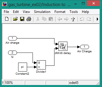
- As you can see in the above image, we have 2 inputs to this system. First one is Air charge and second one is running speed of the turbine.
- If you closely observe the image then, you will notice that we have place 2 inputs to control model named as 'Divide1'. It is actually a comparator and it is continuously comparing the actual running speed of the turbine and the constant reference value.
- Whenever speed will deviate from its reference value then error will be generated.
- Both these inputs goes to the next control box which is, 'variable time delay'. It continuously monitors the ratio of air charge flowing into the system and the corresponding turbine speed. For example, whenever the pressure or temp of the inlet steam will vary then, turbine speed will vary and this control model will generate an error, which will tell us that some abnormalities are going on in the system.
- Next comes the 'Engine Torque Control' . It has 2 inputs. First input is of the Air Charge and the second input is the speed of the Turbine. If you double click on this control model then, a new window will open representing its properties. That window is shown in the image below:
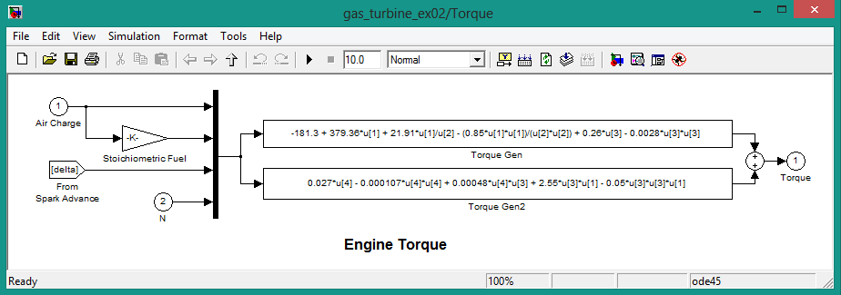
- Engine Torque is defined by 4 input parameters. First is Air charge and you can see that Air Charge input also goes to the Stoichiometric Fuel burning mechanism of combustion chamber. This is because the combustion chamber burns the fuel according to already existing temp and pressure of the charged air.
- If the temp of the air entering the combustion chamber is much low then, it will have to burn more fuel to get the proper temp and pressure of the air.
- Third input is of the 'Spark Advance'. It monitors that either spark plug is igniting the fuel with proper timing or not. If the spark plug doesn't ignite the fuel on exact time then, unburnt fuel particles will comes through exhaust hole. and engine will not run smoothly.
- Fourth input is of the speed of the turbine. Engine Torque control also monitors the existing speed of the turbine. and turbine is not running with the proper speed then, it will decide either it has to open more fuel to get it to proper speed or there is some issue going with spark ignition system.
- All these parameters define the Engine's torque and if there is any problem with any of the input then output torque will also vary accordingly.
- All these system's output goes to the Function Block Parameters and this block converts angular velocity to rpm. It is in fact a techogenerator.
- Techogenerator is in fact a sensor, which is mounted in the shaft of any rotating mechanism and it records the angular speed of the shaft and generates a electrical signal in form of RPMs. It continuously monitors the angular speed of the turbine and then it converts it to RPM.
- In the next stage, output of techogenerator goes to the summing junction. This junction has 2 inputs. First input is from techogenerator and the second input is from external disturbance.
- External Disturbance has a very important role in defining the safe operation of any system. It not only disturbs the system but in severe conditions, it can also collapse the system.
- In the next and final stage, we have a Gear Box model of the Gas turbine. If we double click on it then a new window will open, which will be representing its internal parameters. The internal detail of this control model is shown in the image given below:
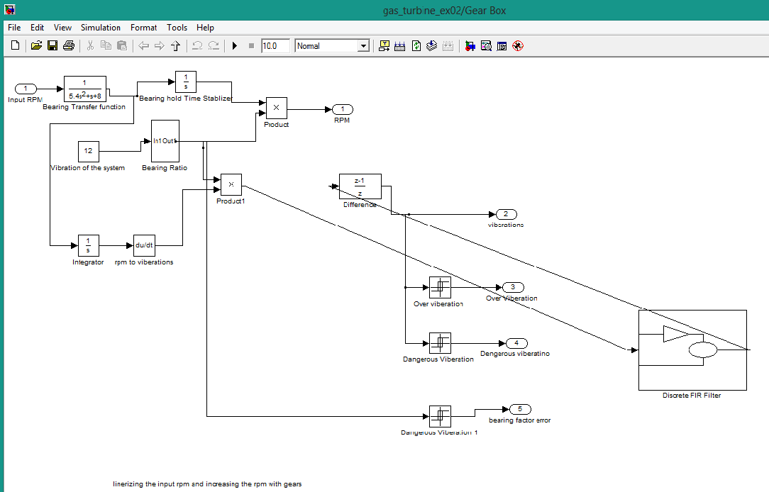
- It is the most important control model of Gas Turbine. It has only one input which is rpm of turbine and this input is coming from techogenerator.
- As you can see in the above given image that, it monitors RPM, Vibrations, Over Vibrations, Dangerous Vibrations and Bearing factor errors.
- Now if you note from the above given image then you will see that RPM, we have connected a scope and the factors which needs continuous monitoring are over vibrations and Bearing Factor error.
- When we will run the simulation, the the system will monitor it completely from first stage to final stage (which is from inlet fresh air to RPM of Gas Turbine) . If any problem comes in the system then turbine speed will vary.
- Dear friends, the beauty of any project's simulation is that we can put abnormalities in our system and then, we can monitor the system's behaviour under these abnormalities. This thing helps in improvising new technology and also lead us to a better design of the system.
- Now in the above figure, we hava a control model named 'variation of the system'. when you will double click on that then, a third small window will open, which is shown in the image given below:
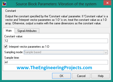
- If you look closely the option named "Constant value" then here we can change the vibrations inserted in the system. Here we change the value according to our own choice and we will start from 1 and then go to maximum value (12) and observe the behaviour of Gas Turbine.
- Now i am going to create some abnormalities on the above system's and we will see their results and then we will conclude either they are dangerous or not.
RESULTS
- We have seen the detailed explanation of "Fault Detection of Gas turbine in MATLAB" and I hope till now you got much familiar with how its operating. So now lets have a look at the results of this simulation.
- First of all, i am going to keep vibrations of the system at 1 then i will play the simulation then the Gear Box will generate the following results, as shown in the image below:
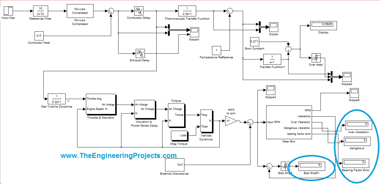
- Now we can see that as we have set the vibration value to 1 so there's no errors gennerated by the simulation. In other words, our gas turbine is running smoothly and is not generating any erros.
- Now i am going to increase the vibrations of the system and i am going to keep its value 10.Then the generated results are given as:
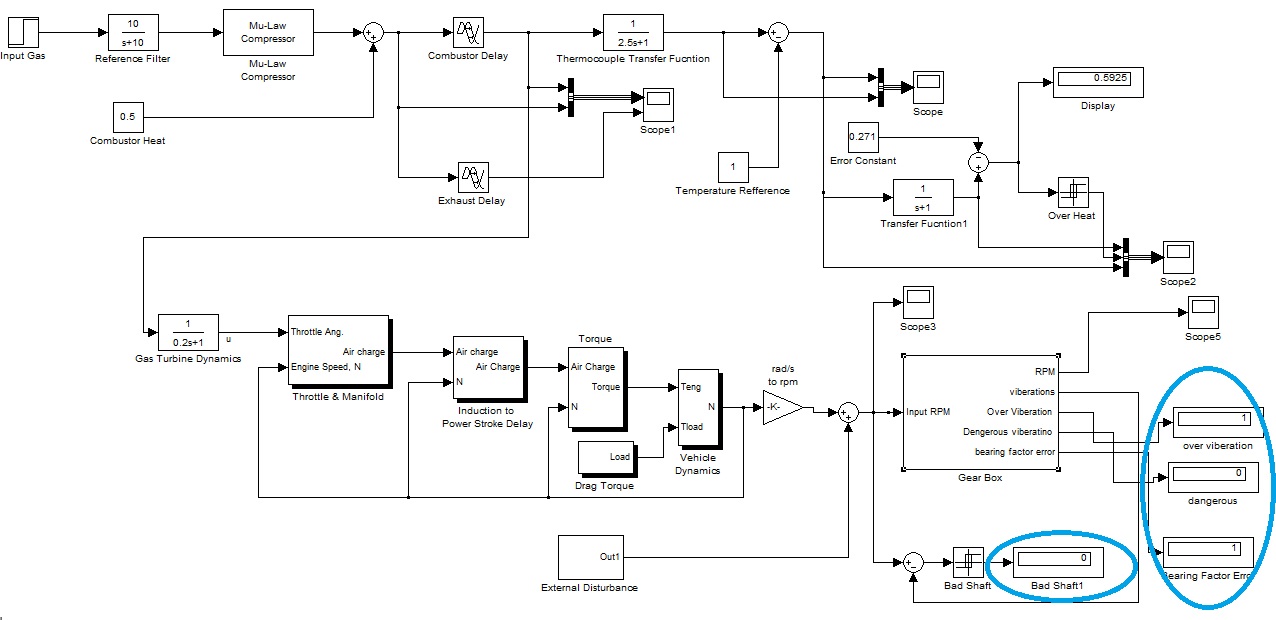
- From above figure, you have seen that System is generating over speeding error and Bearing Factor error but they are not Dangerous yet and system can also run under these conditions.
- In the next stage, i am going to increase the vibrations of systems a little more and i will make its value 12. Now we will observe the output of the system from the below figure:
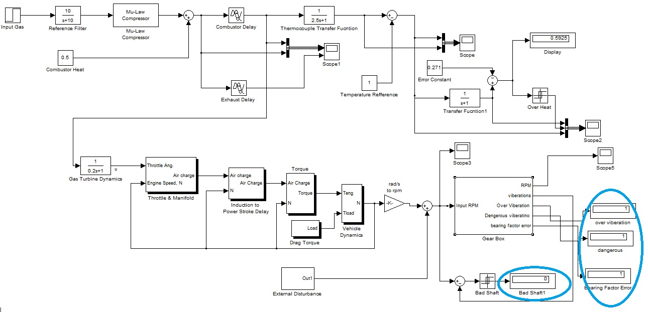
- From above figure, we can easily see that i have increase the vibrations of the turbine upto that extend that it has generated the Dangerous alarm. Now we must immediately stop the system and if we didn't do that, then the system will collapse.
- Now i am going to share the graphs of the no. of Scopes we have added in our system.
- Output graph of "Scope # 1" is given in the figure below:
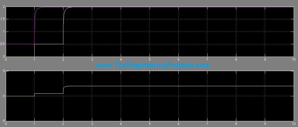
- Above graph is of scope#1 and it is representing the curves of 'Combustor Delay' and 'Exhaust Delay'.
- The output graph of the next scope, added in the system is given in the image below:
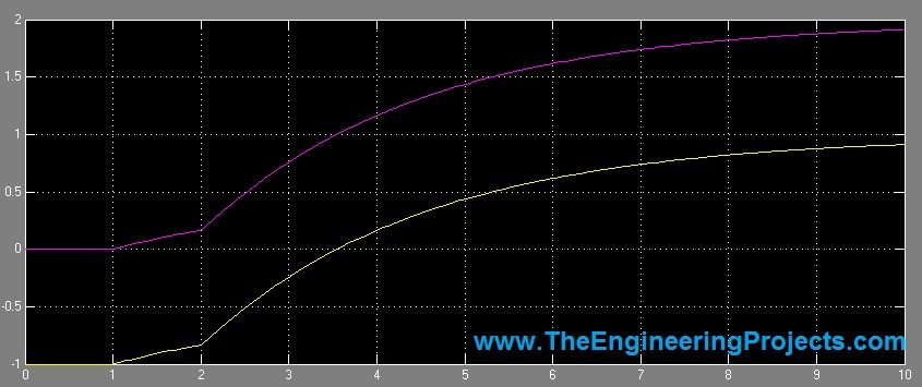
- The above figure is showing the curves of 2 different functions. First is Thermocouple Transfer Function and the next is of Temperature Reference.
- The output graph of the scope#2 is shown in the image below:
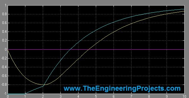
- In the above graph, we have 3 curves. Straight curve is of HEAT. Since turbine is running at normal temp and no over heating is produced in it.
- The green curve is of Combustion delay and Exhaust Delay. This is a very abrupt curve. To make it smooth,we have added another control model named as "Transfer Function 1". That's why the yellow curve is the final curve and it is rather smooth than the other two.
- Now in the end, i am going to share the output curve of scope#5, which is shown as below:
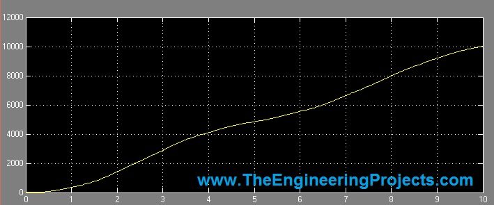
- The above graph is of the RPM of the turbine. As we can see that in the begining, when the simulation was OFF then, curve was at zero. Then we started the simulation and the infact turbine started and it started to accelerate and it gained it max speed which is 10,000 rpm within 10 seconds. which can be verified from above image.


