Financial Calculations in MATLAB


After that I calculated Expected Returns & Covariance Matrix for all these data for the last 10 years and finally plot them. Moreover, I have also plotted the frontiers with risk free rate of 3% so that the ideal and realistic conditions can be compared. So, here are the overall steps we are gonna cover in this project:
- Step 1: Getting Historical Stock Data
- Step 2: Conversion of currencies
- Step 3: Calculate Expected Returns & Covariance Matrix
- Step 4: Plotting 11 different frontiers in one figure
- Step 5: Plotting frontiers with risk free rate of 3%.
You may also like to read:
Step 1: Getting Historical Stock Data
- First of all, I chose 7 financial stock indices for different markets or sectors. So, I used a function named hist_stock_data. The syntax of this function is as follows:
Stocks = hist_stock_data('X', 'Y', 'Z', 'frequency', 'm')
- X is the starting date and is a string in the format ddmmyyyy.
- Y is the ending date and is also a string in the format ddmmyyyy.
- Z is the Ticker symbol, whose historical stock data is needed to be retrieved.
- M denotes that the function will return historical stock data with a frequency of months.
snp500 = hist_stock_data('01111993','01112013','^GSPC','frequency','m'); NDX=hist_stock_data('01111993','01112013','^NDX','frequency','m'); GSPTSE=hist_stock_data('01111993','01112013','^GSPTSE','frequency','m'); DAX = hist_stock_data('01111993','01112013','^GDAXI','frequency','m'); CAC40=hist_stock_data('01111993','01112013','^FCHI','frequency','m'); FTAS=hist_stock_data('01111993','01112013','^FTAS','frequency','m'); SSMI=hist_stock_data('01111993','01112013','^SSMI','frequency','m');
Step 2: Conversion of currencies
The first two values were in US dollars, while third one was in CAD dollars, fourth and fifth values were in Euros, sixth were in GBP and the last one was in Swiss France. Hence, there was a need to convert all these currencies into one currency as instructed. I converted all of them into US dollars. In order to convert them, I first defined the exchange rate between these currencies and the US dollars using the below code:
GBP2USD=1.6; EURO2USD=1.34; CAD2USD=0.95; SF2USD=1.08;After defining the exchange rate, I applied it to all the currencies using the below code:
GSPTSE=CurrencyConvert(GSPTSE, CAD2USD); DAX=CurrencyConvert(DAX, EURO2USD); CAC40=CurrencyConvert(CAC40, EURO2USD); FTAS=CurrencyConvert(FTAS, GBP2USD); SSMI=CurrencyConvert(SSMI, SF2USD);Now all the currencies for the financial stock indices for 7 sectors are obtained in US dollars.
Step 3: Calculate Expected Returns & Covariance Matrix
In this part, we calculated the expected returns and covariance matrix in annual steps for a period of 10 years. I used the data for 7 markets or sectors were obtained in the first step and calculated their expected returns and covariance matrix. The expected rate of return is a probability-weighted average of the rates of return in each scenario. We may write the expected return as:
Where,- p(s) = Probability of each scenario
- r(s) = Holding-price return in each scenario.
- s = number of scenarios.
- n = Maximum number of scenarios.
First of all, I initialized a column matrix and filled it with the above data and took log of each data separately by using MATLAB commands as follows:
covmat=cell(1,11); ret=flipud([log(SSMI.Close) log(FTAS.Close) log(CAC40.Close) log(DAX.Close) log(GSPTSE.Close) log(snp500.Close) log(NDX.Close)]);
Further, I calculated the differences between adjacent elements of each data using the diff command in MATLAB.
logRet=[diff(ret(:,1)) diff(ret(:,2)) diff(ret(:,3)) diff(ret(:,4)) diff(ret(:,5)) diff(ret(:,6)) diff(ret(:,7))];
Expected return is nothing other than a guaranteed rate of return. However, it can be used to forecast the future value of a market, and it also provides a guide from which to measure actual returns. Hence to calculate the expected return, I first take two indices with w as a variable where w = 1:10 and calculated these indices for all the values of w and finally took mean value of each data with these two indices as follows:
ind=[(w-1)*12+1 (w+10)*12]; estReturn(w,:)=[mean(logRet(ind(1):ind(2),1)) mean(logRet(ind(1):ind(2),2)) mean(logRet(ind(1):ind(2),3)) mean(logRet(ind(1):ind(2),4)) mean(logRet(ind(1):ind(2),5)) mean(logRet(ind(1):ind(2),6)) mean(logRet(ind(1):ind(2),7))];
The above values calculated for all the 10 times and hence it is placed within a for loop. estReturn gives us the estimated return for a single month and now there’s a need to convert it to annual return, which is accomplished by below command, simply by mutilpying it with 12.
estReturn(w,:)=estReturn(w,:)*12;
After the calculation of expected return annually, I used the command var(X) to calculate the variance of the data. Although it was not asked to calculate in the problem but in order to calculate the covariance, it is required to first obtain the data such that each row of the matrix becomes an observation and each column is a variable. The command used for the calculation of variance is as shown below:
stdRet(w,:)=sqrt(12*var([ logRet(ind(1):ind(2),1) logRet(ind(1):ind(2),2) logRet(ind(1):ind(2),3) logRet(ind(1):ind(2),4) logRet(ind(1):ind(2),5) logRet(ind(1):ind(2),6) logRet(ind(1):ind(2),7)]));
Finally, I used the MATLAB command cov(x) to calculate the covariance of the data. The syntax used is:
Y = cov(X)Where,
- X = Matrix of data whose covariance is required.
- Y = Covariance of data X.
| Expected Return | SSMI | FTAS | CAC40 | DAX | GSPTSE | SNP50 | NDX |
| 1st year | 0.0625 | 0.0373 | 0.0524 | 0.0632 | 0.0700 | 0.0848 | 0.0644 |
| 2nd year | 0.0954 | 0.0531 | 0.0762 | 0.0846 | 0.0884 | 0.0921 | 0.1290 |
| 3rd year | 0.0872 | 0.0506 | 0.0972 | 0.0940 | 0.0915 | 0.0763 | 0.1004 |
| 4th year | 0.0742 | 0.0457 | 0.0814 | 0.0925 | 0.0747 | 0.0610 | 0.0835 |
| 5th year | 0.0006 | -0.0064 | 0.0122 | 0.0147 | 0.0321 | -0.0058 | 0.0110 |
| 6th year | -0.0112 | 0.0007 | -0.0039 | 0.0103 | 0.0537 | -0.0055 | 0.0115 |
| 7th year | -0.0144 | -0.0069 | -0.0356 | 0.0115 | 0.0494 | -0.0148 | -0.0307 |
| 8th year | -0.0314 | -0.0034 | -0.0573 | -0.0041 | 0.0295 | -0.0048 | -0.0080 |
| 9th year | 0.0081 | 0.0180 | -0.0209 | 0.0359 | 0.0454 | 0.0198 | 0.0470 |
| 10th year | 0.0431 | 0.0529 | 0.0228 | 0.0907 | 0.0644 | 0.0575 | 0.1007 |
Table 1: Expected Returns for 10 years
| Covariance Matrix for 1st year | ||||||
| SSMI | FTAS | CAC40 | DAX | GSPTSE | SNP50 | NDX |
| 0.0334 | 0.0191 | 0.0285 | 0.0324 | 0.0168 | 0.0190 | 0.0196 |
| 0.0191 | 0.0201 | 0.0234 | 0.0271 | 0.0155 | 0.0169 | 0.0257 |
| 0.0285 | 0.0234 | 0.0434 | 0.0444 | 0.0211 | 0.0226 | 0.0380 |
| 0.0324 | 0.0271 | 0.0444 | 0.0609 | 0.0252 | 0.0280 | 0.0527 |
| 0.0168 | 0.0155 | 0.0211 | 0.0252 | 0.0268 | 0.0198 | 0.0342 |
| 0.0190 | 0.0169 | 0.0226 | 0.0280 | 0.0198 | 0.0234 | 0.0379 |
| 0.0196 | 0.0257 | 0.0380 | 0.0527 | 0.0342 | 0.0379 | 0.1411 |
| Covariance Matrix for 2nd year | ||||||
| SSMI | FTAS | CAC40 | DAX | GSPTSE | SNP50 | NDX |
| 0.0318 | 0.0179 | 0.0273 | 0.0322 | 0.0162 | 0.0185 | 0.0235 |
| 0.0179 | 0.0180 | 0.0213 | 0.0258 | 0.0151 | 0.0161 | 0.0269 |
| 0.0273 | 0.0213 | 0.0404 | 0.0427 | 0.0209 | 0.0219 | 0.0390 |
| 0.0322 | 0.0258 | 0.0427 | 0.0590 | 0.0255 | 0.0279 | 0.0503 |
| 0.0162 | 0.0151 | 0.0209 | 0.0255 | 0.0265 | 0.0193 | 0.0367 |
| 0.0185 | 0.0161 | 0.0219 | 0.0279 | 0.0193 | 0.0230 | 0.0394 |
| 0.0235 | 0.0269 | 0.0390 | 0.0503 | 0.0367 | 0.0394 | 0.1014 |
| Covariance Matrix for 3rd year | ||||||
| SSMI | FTAS | CAC40 | DAX | GSPTSE | SNP50 | NDX |
| 0.0314 | 0.0181 | 0.0280 | 0.0320 | 0.0164 | 0.0186 | 0.0237 |
| 0.0181 | 0.0181 | 0.0214 | 0.0261 | 0.0152 | 0.0160 | 0.0270 |
| 0.0280 | 0.0214 | 0.0397 | 0.0433 | 0.0212 | 0.0224 | 0.0399 |
| 0.0320 | 0.0261 | 0.0433 | 0.0579 | 0.0259 | 0.0282 | 0.0509 |
| 0.0164 | 0.0152 | 0.0212 | 0.0259 | 0.0266 | 0.0194 | 0.0371 |
| 0.0186 | 0.0160 | 0.0224 | 0.0282 | 0.0194 | 0.0227 | 0.0395 |
| 0.0237 | 0.0270 | 0.0399 | 0.0509 | 0.0371 | 0.0395 | 0.1014 |
Step 4: Plotting 11 different frontiers in one figure
In this part, it was asked to plot the 11 different frontiers in one figure. The concept of efficient frontier was introduced by Harry Markowitz and it is defined as if a portfolio or a combination of assets has the best expected rate of return for the level of risk, it is facing, then it will be referred as “efficient”.
Few more MATLAB Projects:
- Find Roots of Quadratic Equation
- Send Data to Serial Port in MATLAB
- Speech Recognition using Correlation
- DTMF Decoder using MATLAB
- Hexapod Simulation in MATLAB
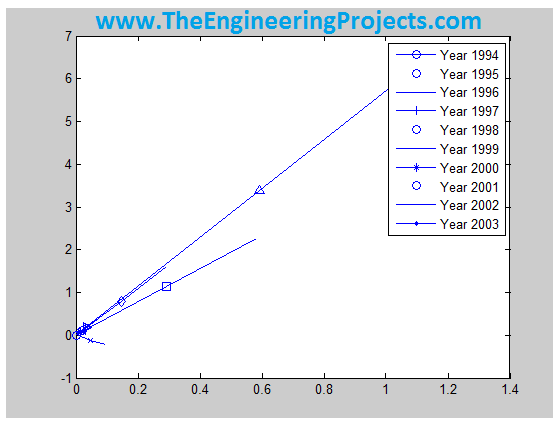
In order plot them, I used the below code in MATLAB, I used different markers for different plots so that they could be distinguished from one another quite easily. Moreover, I used the command legend in order to show the respective years for which the graphs are plotted. RF is a variable which indicate the risk-free rate and as it is asked to operate under efficient frontier that’s why risk-free rate is equal to zero.
RF=0; for w=1:10 [xopt(:,w), muopt(w), sigopt(w)] = highest_slope_portfolio( covmat{1,w}, RF, estReturn(w,:)', stdRet(w,:) ); end mker=['o' '+' '*' '.' 'x' 's' 'd' '^' '>' '<'] figure for w=1:10 plot (sigopt(w), muopt(w) ,'Marker', mker(w)); hold on; plot (0, RF, 'o'); hold on; RF_p1 = [0 sigopt(w) 2* sigopt(w)]; opt1_p = [.02 muopt(w) (2 * muopt(w) - RF) ]; line(RF_p1, opt1_p ); end legend('Year 1994', 'Year 1995', 'Year 1996', 'Year 1997','Year 1998','Year 1999','Year 2000', 'Year 2001', 'Year 2002', 'Year 2003')In this code, first of all I used highest_slope_portfolio function. This function finds the portfolio with the highest slope. Results are shown in the below figure annually:

Step 5: Plotting frontiers with risk free rate of 3%
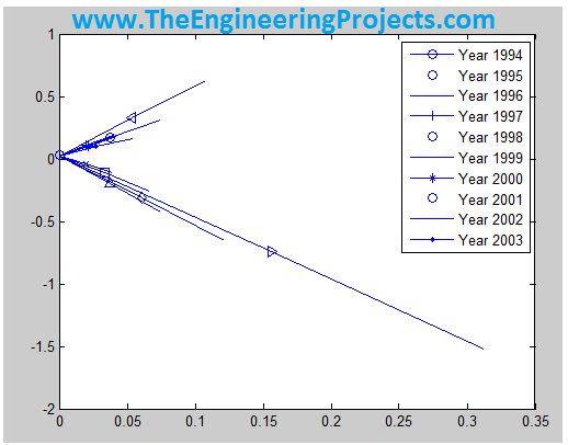
The plot in Part (c) was about the efficient frontier with risk rate equal to zero i.e. operating in an ideal condition while in this part, it was asked to plot the same graphs but this time include a risk-free rate of 3%. Hence I used the same code as for the previous part but only this time I used RF = 0.03 as I needed to include a risk free rate of 3%. The code used in MATLAB for this part is shown below:
RF=0.03; %the risk free rate for w=1:10 [xoptRF{w}, muoptRF(w), sigoptRF(w)] = highest_slope_portfolio( covmat{1,w}, RF, estReturn(w,:)', stdRet(w,:) ); end figure for w=1:10 plot (sigoptRF(w), muoptRF(w) ,'Marker', mker(w)); hold on; plot (0, RF, 'o'); hold on; RF_p1 = [0 sigoptRF(w) 2* sigoptRF(w)]; opt1_p = [.02 muoptRF(w) (2 * muoptRF(w) - RF) ]; line(RF_p1, opt1_p ); end legend('Year 1994', 'Year 1995', 'Year 1996', 'Year 1997','Year 1998','Year 1999','Year 2000', 'Year 2001', 'Year 2002', 'Year 2003')
The result for this part i.e. after including a risk-free rate of 3% is shown in the figure below. If the Figure 1 and Figure 2 are closely examined then one can see the clear difference. When the risk-free rate was considered zero, all the expected estimate graphs were in positive direction depicting the profit annually while after adding a risk-free rate of 3%, few of the graphs went in the negative direction depicting the loss in those years. Hence adding the risk factor may cause the business to get deceased and it may even cause it to decline continuously which results in disaster.

That's all for today, in the coming post, I will calculate more financial terms like Optimal asset allocation, average return, standard deviation and much more, so stay tuned and have fun.


