Analysis of Sinusoidal Pulse Width Modulation of AC Signal

Pulse Width Modulation or PWM is a technique which is used for getting Analog Results with digital means. We can say that some Digital Control or some Electronics algorithm is used to generate square waves. Square wave is in fact a signal which is generated through switching between ON & OFF states. There are no of ways to generate PWM. For example in modern electronics projects PWM is generated through some type of micro controllers or 555 Timers. If you recall my previous project tutorials, in which I have generated PWM through 555 timer. Since in this tutorial we are working with-in MATLAB premises so we will only discuss CODE and no hardware design involved in this tutorial. Now without wasting any time, I think we should move towards the CODE of the project. Stay tuned and believe me you will learn something new from this project.

You should also read:

• How to Create a GUI in MATLAB?
• Protect Code in M File
• Protect Simulink Design in Matlab

Analysis of Sinusoidal Pulse Width Modulation of an AC Signal

• First of all open your MATLAB software and a command window will appear. Now first thing to do is to clear the command window and remove all the previous variables or functions from MATLAB.

• This is done through MATLAB language and we have commands to do this. The commands are given below:

clc clear all disp('Sinusoidal Pulse Width Modulation of AC Signal') disp(' ')

• 'clc' and 'clear all' command will clear the command window and remove all the variables already existing.
• Then the next command is 'disp(' ')' , and this command is used to display anything in command window. In dispaly command i have written the title of my project, which is "Sinusoidal Pulse Width Modulation of AC Signal" .
• Now coming towards part 2, which is to enter some information from user side. Since we are analyzing the PWM of AC signal and we need to enter the data of that particular signal, which we are going to analyze.
• The code to do all this is given below:

Vrin=1; f=input('The frequency of the input supply voltage, f = '); Z=1; ma=input('the modulation index,ma, (0<ma<1), ma = '); phi=input('the phase angle of the load in degrees = '); Q=input('The number of pulses per half period = ');

• The first command is 'Vrin' which is RMS value of the supply voltage in Per Unit. As you know that the maximum value of Per Unit is one, so i have kept its value equals to 1.
• In the next steps, you can see that i have given the 'input' command. This command is used at that place if we need data from external source, which means if user will enter that data according to the input signal.
• As you can see in the above code that Firstly it is asking frequency then comes the variable 'Z', which is load impedence in per-unit and we have kept its value 1.
• 'ma' is the modulation index and its value varies from 0 to 1.
• 'phi' is the phase angle of load in degrees.
• 'Q' is the no. of pulses per half period of the given cycle. MATLAB code will ask these values from user to enter them manually according to the that signal, which is under consideration.
• Coming towards the Third part of the CODE, which is to calculate load parameters. The parameters of the load signal which we have entered in the above commands (part 2).
• MATLAB Commands to calculate phase angle, Resistance and Inductance of the the load are given below:

phi=phi*pi/180; R=Z*cos(phi); L=(Z*sin(phi))/(2*pi*f);

• 'phi' is the load phase angle in degrees. while the other 'pi' is a built-in MATLAB function. In MATHEMATICS pi has a constatnt value which is '2.14' .
• Next 2 formulas the used to calculate Resistance(R) and Inductance(L) of the load respectively.
• Up till now we have entered the known values of the signal under examination. No in the next part of the tutorial, we are going to calculate the no of pulses per period of the sine wave or AC Signal under consideration.
• MATLAB command to calculate the period of an AC signal is given below:

N=2*Q;

• This is a simple product formula. 'Q' is the no of pulses per half period and when we will multiply it with 2, we get no of pulses in full period, which is 'N'.
• Period of an AC cycle can be defined as the time taken by the AC voltage to complete its one cycle. Period is reciprocal of Frequency. Frequency can be defined as the no of waves passing through a particular point in one second. Both these terms are necessary to explain AC signal.
• In the next part of the code, we are going to develop a function to generate a saw-tooth voltage from the given input parameters of the signal.
• In each period of the sawtooth, there is one increasing and decreasing part of the sawtooth, thus the period of the input supply is divided into into 2N sub-periods. The function to develop this sawtooth voltage is given below:

for k=1:2*N for j=1:50 i=j+(k-1)*50; wt(i)=i*pi/(N*50); Vin(i)=sqrt(2)*Vrin*sin(wt(i)); ma1(i)=ma*abs(sin(wt(i))); if rem(k,2)==0 Vt(i)=0.02*j; if abs(Vt(i)-ma*abs(sin(wt(i))))<=0.011 m=j; beta(fix(k/2)+1)=3.6*((k-1)*50+m)/N; else j=j; end else Vt(i)=1-0.02*j; if abs(Vt(i)-ma*abs(sin(wt(i))))ma*abs(sin(wt(i))) Vout(i)=0; else Vout(i)=Vin(i); end end end beta(1)=[];

• The above part code seems to be bit lengthy but it is not that difficult to understand. Since in the previous part we have generated a saw-tooth voltage and we need to calculate its period.
• To calculate period, we have introduced some counters in our code named i,j and k. 'i' is the generalized counter.
• 'k' is the counter, used to count sub-periods and 'j' is the counter inside these sub-periods. From the beginning of the above part, we have defined a generalized counter, then we have calculated supply voltages through modulation of index.

• Send Data to Serial Port in MATLAB
• Speech Recognition using Correlation
• DTMF Decoder using MATLAB
• Hexapod Simulation in MATLAB

• Then i have written a conditional loop consisting of 'if' and 'else' and we have generated a saw-tooth waveform from it.
• In the end, the final value of this saw-tooth voltage is saved in variable named 'beta'.
• Up-til now we have generated a saw-tooth voltage and we have calculated the beginning value (alpha) ,ending value (beta) and the period (width) of this saw-tooth voltage.
• Now in the next part we will write the command to display all these values of the saw-tooth voltage curve. Part of CODE is given below:

disp(' ') disp('......................................................................') disp('alpha beta width') [alpha' beta' (beta-alpha)']

• In this step, we will simply display the values of the saw-tooth voltage, which we have generated in the above code.
• Now we will write a CODE to plot the graphs of the the voltage curve, we have generated above:

a=0; subplot(3,1,1) plot(wt,Vin,wt,a) axis([0,2*pi,-2,2]) title('Generation Of The Output Voltage Pulses ') ylabel('Vin(pu)'); subplot(3,1,2) plot(wt,Vt,wt,ma1,wt,a) axis([0,2*pi,-2,2]) ylabel('Vt, m(pu)'); subplot(3,1,3) plot(wt,Vout,wt,a) axis([0,2*pi,-2,2]) ylabel('Vo(pu)'); xlabel('Radian');

• The title of this graph is generation of output voltage pulses and it will plot the graphs.
• In next step, we will examine the output voltage curve. Its RMS value. HARMONIC components present in it and THRESHOLD value. CODE to examine all this is:

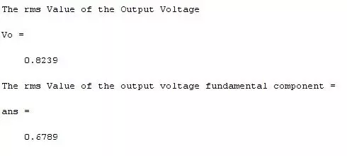
Vo =sqrt(1/(length(Vout))*sum(Vout.^2)); disp('The rms Value of the Output Voltage ') Vo y=fft(Vout); y(1)=[]; x=abs(y); x=(sqrt(2)/(length(Vout)))*x; disp('The rms Value of the output voltage fundamental component = ') x(1) THDVo = sqrt(Vo^2 -x(1)^2)/x(1);

• The formulas to calculate all these parameters of output voltage curve are given in the above code.
• Uptil now, we have calculated all the parameters of output voltage curve and now i am going to calculate the current parameters of the output curve. The algorithm to calculate the output current wave-form is given below:

m=R/(2*pi*f*L); DT=pi/(N*50); C(1)=-10; i=100*N+1:2000*N; Vout(i)=Vout(i-100*N*fix(i/(100*N))+1); for i=2:2000*N; C(i)=C(i-1)*exp(-m*DT)+Vout(i-1)/R*(1-exp(-m*DT)); end

• Now we are going to calculate all the parameters of the current waveform, which we previously explained for the output voltage waveform. Now we are going to calculate the RMS value, Harmonic component and Threshold value of the output current. CODE to do all this is given below:

for j4=1:100*N CO(j4)=C(j4+1900*N); CO2= fft(CO); CO2(1)=[]; COX=abs(CO2); COX=(sqrt(2)/(100*N))*COX; end CORMS = sqrt(sum(CO.^2)/(length(CO))); disp(' The RMS value of the load current is') CORMS THDIo = sqrt(CORMS^2-COX(1)^2)/COX(1);

• All the above data and results were to monitor output parameters.
• Now we are going to calculate the current parameters of input supply voltages.
• first of all, i will find the input supply current and then i will analyze this supply current. Find its RMS value, Find its Fourier series, its displacement factor and Threshold value of the input supply current. The CODE to perform all this work simultaneously is given below:

for j2=1900*N+1:2000*N if Vout(j2)~=0 CS(j2)=C(j2); else CS(j2)=0; end end for j3=1:100*N CS1(j3)=CS(j3+1900*N); end CSRMS= sqrt(sum(CS1.^2)/(length(CS1))); disp('The RMS value of the supply current is') CSRMS CS2= fft(CS1); CS2(1)=[]; CSX=abs(CS2); CSX=(sqrt(2)/(100*N))*CSX; THDIS = sqrt(CSRMS^2-CSX(1)^2)/CSX(1); phi1 = atan(real(CS2(1))/imag(CS2(1)))-pi/2; PF=cos(phi1)*CSX(1)/CSRMS;

• Up till now we have calculated all the parameters and now we are going to draw a table in MATLAB and it will show all the results simultaneously.
• The combined code to display all the parameters on the output window is given below:

disp(' Performance parameters are') THDVo THDIo THDIS PF a=0; figure(2) subplot(3,2,1) plot(wt,Vout(1:100*N),wt,a); title(''); axis([0,2*pi,-1.5,1.5]); ylabel('Vo(pu)'); % subplot(3,2,2) plot(x(1:100)) title(''); axis([0,100,0,0.8]); ylabel('Von(pu)'); subplot(3,2,3) plot(wt,C(1900*N+1:2000*N),wt,a); title(''); axis([0,2*pi,-1.5,1.5]); ylabel('Io(pu)'); subplot(3,2,4) plot(COX(1:100)) title(''); axis([0,100,0,0.8]); ylabel('Ion(pu)'); subplot(3,2,5) plot(wt,CS(1900*N+1:2000*N),wt,a); axis([0,2*pi,-1.5,1.5]); ylabel('Is(pu)'); xlabel('Radian'); subplot(3,2,6) plot(CSX(1:100)) title(''); axis([0,100,0,0.8]); ylabel('Isn(pu)'); xlabel('Harmonic Order');

• In the above code 2 commands are used in excess. First one is 'plot', which is used to plot any particular function in MATLAB and the second command is 'subplot' which is used to draw multiple plots like 2 or 3 plots in the same window.
• When you will write all this CODE and you will run it then, graphs will appear according to the data you entered to examine that particular signal.

RESULTS

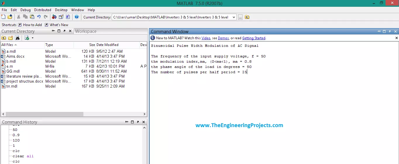
• The graphical results of all the above tutorial will be displayed in this section. First of all, when you will run the M-file then command window will appear and it will ask you give some input values of the supply voltages.
• Such command window is shown in the image below:

•  After inputing these values, the above given algorithm will start plotting the graphs, the firsst graph is shown in the below figure:

•  Next plot is shown below, the graphs are labelled that's why I am not explaining them much.

• It will also give some other values in the MATLAB's command window, a screenshot of these values is as follows:

• Here's the complete programming code for this project:

clc clear all disp('Sinusoidal Pulse Width Modulation of AC Signal') disp('  ') Vrin=1; f=input('The frequency of the input supply voltage, f = '); Z=1; ma=input('the modulation index,ma, (0<ma<1), ma = '); phi=input('the phase angle of the load in degrees = '); Q=input('The number of pulses per half period = '); phi=phi*pi/180; R=Z*cos(phi); L=(Z*sin(phi))/(2*pi*f); N=2*Q; for k=1:2*N for j=1:50 i=j+(k-1)*50; wt(i)=i*pi/(N*50); Vin(i)=sqrt(2)*Vrin*sin(wt(i)); ma1(i)=ma*abs(sin(wt(i))); if rem(k,2)==0 Vt(i)=0.02*j; if abs(Vt(i)-ma*abs(sin(wt(i))))<=0.011 m=j; beta(fix(k/2)+1)=3.6*((k-1)*50+m)/N; else j=j; end else Vt(i)=1-0.02*j; if abs(Vt(i)-ma*abs(sin(wt(i))))<0.011 l=j; alpha(fix(k/2)+1)=3.6*((k-1)*50+l)/N; else j=j; end end if Vt(i)>ma*abs(sin(wt(i))) Vout(i)=0; else Vout(i)=Vin(i); end end end beta(1)=[]; disp('  ') disp('..........................................') disp('alpha    beta    width') [alpha'  beta'  (beta-alpha)'] a=0; subplot(3,1,1) plot(wt,Vin,wt,a) axis([0,2*pi,-2,2]) title('Generation Of The Output Voltage Pulses ') ylabel('Vin(pu)'); subplot(3,1,2) plot(wt,Vt,wt,ma1,wt,a) axis([0,2*pi,-2,2]) ylabel('Vt, m(pu)'); subplot(3,1,3) plot(wt,Vout,wt,a) axis([0,2*pi,-2,2]) ylabel('Vo(pu)'); xlabel('Radian'); Vo =sqrt(1/(length(Vout))*sum(Vout.^2)); disp('The rms Value of the Output Voltage ') Vo y=fft(Vout); y(1)=[]; x=abs(y); x=(sqrt(2)/(length(Vout)))*x; disp('The rms Value of the output voltage fundamental component = ') x(1) THDVo = sqrt(Vo^2 -x(1)^2)/x(1); m=R/(2*pi*f*L); DT=pi/(N*50); C(1)=-10; i=100*N+1:2000*N; Vout(i)=Vout(i-100*N*fix(i/(100*N))+1); for i=2:2000*N; C(i)=C(i-1)*exp(-m*DT)+Vout(i-1)/R*(1-exp(-m*DT)); end for j4=1:100*N CO(j4)=C(j4+1900*N); CO2= fft(CO); CO2(1)=[]; COX=abs(CO2); COX=(sqrt(2)/(100*N))*COX; end CORMS = sqrt(sum(CO.^2)/(length(CO))); disp(' The RMS value of the load current is') CORMS THDIo = sqrt(CORMS^2-COX(1)^2)/COX(1); for j2=1900*N+1:2000*N if Vout(j2)~=0 CS(j2)=C(j2); else CS(j2)=0; end end for j3=1:100*N CS1(j3)=CS(j3+1900*N); end CSRMS= sqrt(sum(CS1.^2)/(length(CS1))); disp('The RMS value of the supply current is') CSRMS CS2= fft(CS1); CS2(1)=[]; CSX=abs(CS2); CSX=(sqrt(2)/(100*N))*CSX; THDIS = sqrt(CSRMS^2-CSX(1)^2)/CSX(1); phi1 = atan(real(CS2(1))/imag(CS2(1)))-pi/2; PF=cos(phi1)*CSX(1)/CSRMS; disp(' Performance parameters are') THDVo THDIo THDIS PF a=0; figure(2) subplot(3,2,1) plot(wt,Vout(1:100*N),wt,a); title(''); axis([0,2*pi,-1.5,1.5]); ylabel('Vo(pu)'); % subplot(3,2,2) plot(x(1:100)) title(''); axis([0,100,0,0.8]); ylabel('Von(pu)'); subplot(3,2,3) plot(wt,C(1900*N+1:2000*N),wt,a); title(''); axis([0,2*pi,-1.5,1.5]); ylabel('Io(pu)'); subplot(3,2,4) plot(COX(1:100)) title(''); axis([0,100,0,0.8]); ylabel('Ion(pu)'); subplot(3,2,5) plot(wt,CS(1900*N+1:2000*N),wt,a); axis([0,2*pi,-1.5,1.5]); ylabel('Is(pu)'); xlabel('Radian'); subplot(3,2,6) plot(CSX(1:100)) title(''); axis([0,100,0,0.8]); ylabel('Isn(pu)'); xlabel('Harmonic Order');