Hello friends! I hope you all had a great start to the new year.
In our first lecture, we had looked at the MATLAB prompt and also learned how to enter a few basic commands that use math operations. This also allowed us to use the MATLAB prompt as an advanced calculator. Today we will look at the various MATLAB keywords, and a few more basic commands and MATLAB functions, that will help us keep the prompt window organized and help in mathematical calculations. We are also going to get familiar with MATLAB’s interface and the various windows. We will also write our first user-defined MATLAB functions.
MATLAB keywords and functions
Like any programming language, MATLAB has its own set of keywords that are the basic building blocks of MATLAB. These 20 building blocks can be called by simply typing ‘iskeyword’ in the MATLAB prompt.
The list of 21 MATLAB keywords obtained as a result of running this command is as follows:
'break'
'case'
'catch'
'classdef'
'continue'
'else'
'elseif'
'end'
'for'
'function'
'global'
'if'
'otherwise'
'parfor'
'persistent'
'return'
'spmd'
'switch'
'try'
'while'
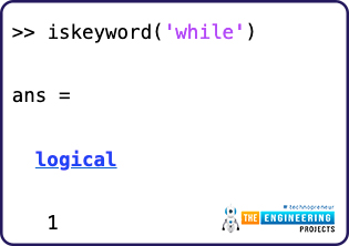
To test if the word while is a MATLAB keyword, we run the command
iskeyword(‘while’)
The output ‘1’ is saying that the result is ‘True’, and therefore, ‘while’ is indeed a keyword.
‘logical’ in the output refers to the fact that this output is a datatype of the type ‘logical’.
Other data types include ‘uint8’, ‘char’ and so on and we will study these in more detail in the next lecture.
Apart from the basic arithmetic functions, MATLAB also supports relational operators, represented by symbols and the corresponding functions which look as follows:
Here, we create a variable ‘a’ which stores the value 1. The various comparison operators inside MATLAB used here, will give an output ‘1’ or ‘0’ which will mean ‘True’ or ‘False’ with respect to a particular statement.
Apart from these basic building blocks, MATLAB engineers have made available, a huge library of functions for various advanced purposes, that have been written using the basic MATLAB keywords only.
We had seen previously that the double arrowed (‘>>’) MATLAB prompt is always willing to accept command inputs from the user. Notice the ‘’ to the left of the MATLAB prompt, with a downward facing arrow. Clicking this downward facing arrow allows us to access the various in-built MATLAB functions including the functions from the various installed toolboxes. You can access the entire list of in-built MATLAB functions, including the trigonometric functions or the exponents, logarithms, etc.
Here are a few commands that we recommend you to try that make use of these functions:
A = [1,2,3,4];
B = sin(A);
X = 1:0.1:10;
Y = linspace(1,10,100);
clc
clear all
quit
Notice that while creating a matrix of numbers, we always use the square braces ‘[]’ as in the first line, whereas, the input to a function is always given with round brace ‘()’ as in the second line.
We can also create an ordered matrix of numbers separated by a fixed difference by using the syntax start:increment:end, as in the third command.
Alternatively, if we need to have exactly 100 equally separated numbers between a start and and end value, we can use the ‘linspace’ command.
Finally, whatever results have been output by the MATLAB response in the command window can be erased by using the ‘clc’ command which stands for ‘clear console’, and all the previously stored MATLAB variables can be erased with the ‘clear all’ command.
To exit MATLAB directly from the prompt, you can use the ‘quit’ command.
In the next section, let us get ourselves familiarized with the MATLAB environment.
The MATLAB Interface Environment
A typical MATLAB work environment looks as follows. We will discuss the various windows in detail:
When you open MATLAB on your desktop, the following top menu is visible. Clicking on ‘new’ allows us to enter the editor window and write our own programs.
You can also run code section by section by using the ‘%%’ command. For beginners, I’d say that this feature is really really useful when you’re trying to optimize parameters.
Menu Bar and the Tool Bar
On the top, we have the menu bar and the toolbar. This is followed by the address of the current directory that the user is working in.
By clicking on ‘New’ option, the user can choose to generate a new script, or a new live script, details of which we will see in the next section.
Current Folder
Under the Current Folder window, you will see all the files that exist in your current directory. If you select any particular file, you can also see it details in the bottom panel as shown below.
Editor Window
The Editor Window will appear when you open a MATLAB file with the extension ‘.m’ from the current folder by double clicking it, or when you select the ‘New Script’ option from the toolbar. You can even define variables like you do in your linear algebra class.
The code in the editor can also be split into various sections using the ‘%%’ command. Remember that a single ‘%’ symbol is used to create a comment in the Editor Window.
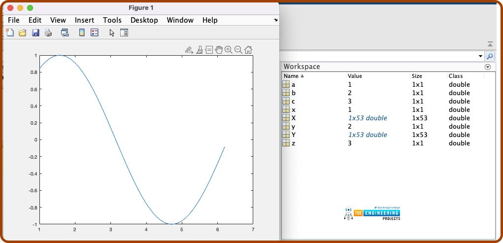
Workspace Window
Remember that the semicolon ‘;’ serves to suppress the output. Whenever you create new variables, the workspace will start showing all these variables. As we can see, the variables named ‘a’, ‘b’, ‘c’, and ‘x’, ‘y’, ‘z’. For each variable, we have a particular size, and a type of variable, which is represented by the ‘Class’. Here, the ‘Class’ is double for simple numbers.
You can directly right click and save any variable, directly from this workspace, and it will be saved in the ‘.mat’ format in the current folder.
Live Editor Window
If however, you open a ‘.mlx’ file from the current folder, or select the option to create a ‘New Live Script’ from the toolbar, the Live Editor window wil open instead.
With the Live Script, you can get started with the symbolic manipulation, or write text into the MATLAB file as well. Live scripts can also do symbolic algebraic calculation in MATLAB.
For example, in the figure below, we define symbol x with the command
syms x
We click ‘Run’ from the toolbar to execute this file.
The Live Editor also allows us to toggle between the text and the code, right from the toolbar. After that, the various code sections can be run using the ‘Run’ option from the toolbar and the rendered output can be seen within the Live Editor.
Command History
Finally, there is the command history window, which will store all the previous commands that were entered on any previous date in your MATLAB environment.
Figure window
Whenever you generate a plot, the figure window will appear which is an interactive window with it’s own toolbar, to interact with the plots.
We use the following commands to generate a plot, and you can try it too:
X = 1:0.1:2*pi;
Y = sin(X)
plot(X,Y)
The magnifier tools help us to zoom into and out of the plot while the ‘=’ tool helps us to find the x and y value of the plot at any particular point.
Also notice that now, the size of the ‘X’ and ‘Y’ variables is different, because we actually generated a matrix instead of assigning a single number to the variable.
Creating a New User-Defined Function
By selecting New Function from the toolbar, you can also create a new user-defined function and save it as an m-file. The name of this m-file is supposed to be the same as the name of the function. The following template gets opened when you select the option to create a new user-defined function:
The syntax function is used to make MATLAB know that what we are writing is a function filee. Again notice that the inputs to the function, inputArg1 and inputArg2, are inside the round braces. The multiple outputs are surrounded by square braces because these can be a matrix. We will create a sample function SumAndDiff using this template, that will output the sum and difference of any two numbers. The function file SumAndDiff.m looks as follows:
Once this function is saved in the current folder, it can be recognized by a current MATLAB script or the MATLAB command window and used.
Exercises:
Create a list of numbers from 0 to 1024, with an increment of 2.
Find the exponents of 2 from 0th to 1024th exponent using results of the previous exercise.
What is the length of this matrix?
Plot the output, and change the y axis scale from linear to log, using the following command after using the plot function: set(gca, ‘yscale’, ‘log’)
Let us go ahead now and import an image into MATLAB to show you what the image looks like in the form of matrices. You need to have the image processing toolbox installed in order for the image functions to work.
Run the following command in the MATLAB prompt:
I = imread(‘ngc6543a.jpg’);
This calls the image titled ‘ngc6543a.jpg’ which is stored inside MATLAB itself for example purposes. Notice the size of this image variable I in the workspace. You will interestingly find this to be a 3D matrix. Also note the class of this variable.
In the next tutorial, we will deep dive into the MATLAB data types, the format of printing these data types and write our first loops inside MATLAB.