

This post is the next part of our previous post Financial Calculations in MATLAB named as Implementation of Black Litterman Approach in MATLAB, so if you haven't read that then you can't understand what's going on here so, its better that you should first have a look at that post. Moreover, as this code is designed after a lot of our team effort so its not free but we have placed a very small cost of $20. So you can buy it easily by clicking on the above button.In the previous post, we have covered five steps in which we first get the financial stock data, then converted it to common currency and after that we calculated the expected returns and covariance matrix and then plot the frontiers with and without risk free rate of 3%. Now in this post, we are gonna calculate the optimal asset allocation, average return after the back test, calculation of alphas and betas of the system and finally the implementation of black-litterman approach. First five steps are explained in the previous tutorial and the next four steps for Implementation of Black Litterman Approach in MATLAB are gonna discuss in this tutorial, which are as follows:
- Step 6: Calculate Optimal Asset Allocation
- Step 7: Average Return after the back test
- Step 8: Calculation of Standard Deviation
- Step 9: Calculate alphas & betas of the system
- Step 10: Implementation of Black Litterman Approach
You may also like to read:
Step 6: Calculate Optimal Asset Allocation
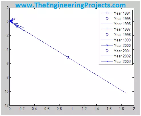
In this part of the problem,I calculated the optimal asset allocation in the different years by choosing a constant required return. I chose the constant required return equal to 0.01 and used the highest_slope_portfolio function and plot the graphs. The code used in MATLAB is shown in the below:
ConsRet=0.010 for w=1:10 [xoptCR(:,w), muoptCR(w), sigoptCR(w)] = highest_slope_portfolio( covmat{1,w}, ConsRet , estReturn(w,:)', stdRet(w,:) ); End
The result for this part is shown in the Figure 3. For a constant required return of 0.01, portfolio turnover for each year has increased approximately by 2%.
Step 7: Average Return after the back test
In this part of the assignment, it was asked to perform a back test for the optimized portfolios and calculate the average return and the standard deviation for this portfolio. Average return is the average of expected return for the corresponding year and it is calculated by the below code in MATLAB, where w is varying from 1 to 10 to calculate for all the 10 years.
BTreturn(w,:)=estReturn(w,:)*xoptCR(:,w);Results obtained after the back test for the optimized portfolios for average return are shown in table3 below:
| Average Return after the back test | |
| 1st year | 0.1158 |
| 2nd year | 0.0889 |
| 3rd year | 0.0797 |
| 4th year | 0.0628 |
| 5th year | -0.0660 |
| 6th year | -0.4323 |
| 7th year | -5.1212 |
| 8th year | -0.6820 |
| 9th year | 0.2891 |
| 10th year | 0.1691 |
Table : Average return after the back test
Step 8: Calculation of Standard Deviation
The standard deviation of the rate of return is a measure of risk. It is defined as the square root of the variance, which in turn is the expected value of the squared deviations from the expected return. The higher the volatility in outcomes, the higher will be the average value of these squared deviations. Therefore, variance and standard deviation measure the uncertainty of outcomes. Symbolically,
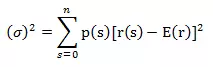
- S = Standard Deviation
- E(r) = Expected return
- p(s) = Probability of each scenario
- r(s) = Holding-price return in each scenario.
- s = number of scenarios.
- n = Maximum number of scenarios.
BTstd(w,:)=sqrt(stdRet(w,:).^2*(xoptCR(:,w).^2));The results of standard deviation for the 10 years are as follows:
| Standard Deviation after the back test | |
| 1st year | 0.2942 |
| 2nd year | 0.1833 |
| 3rd year | 0.1799 |
| 4th year | 0.1733 |
| 5th year | 0.4026 |
| 6th year | 1.5834 |
| 7th year | 16.1279 |
| 8th year | 2.1722 |
| 9th year | 1.0430 |
| 10th year | 0.4949 |
Step 9: Calculate Alphas & Betas of the system
In this part, it was asked to use a broad stock index for testing and check whether our portfolio is in line with the CAPM prediction: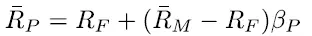
FTLC= hist_stock_data('01111993','01112013','^FTLC','frequency','m'); LRFTLC=diff(log(FTLC.Close));After that I calculated the expected return of one unit of each asset based on the model which gave me the total covariance matrix for the single and multi indexed model. Finally, I calculated the alpha and beta for the model. The MATLAB code used for performing these actions is shown below:
for i = 1:7 mdl_si{i} = LinearModel.fit(LRFTLC, logRet(:,i), 'linear'); mdl_ret_s(i) = mdl_si{i}.Coefficients.Estimate(1:2)' * [1; 12*mean(LRFTLC)]; mdl_cov_s(i) = mdl_si{i}.RMSE^2; alpha_s = [mdl_si{i}.Coefficients.Estimate(1), alpha_s]; beta_s = [mdl_si{i}.Coefficients.Estimate(2), beta_s]; endAs a result, alphas and betas of the system are obtained which are shown in the table below:
| Aplha | Beta |
| 0.0068 | 0.1748 |
| 0.0057 | 0.0335 |
| 0.0050 | 0.0528 |
| 0.0063 | 0.0552 |
| 0.0030 | 0.0249 |
| 0.0035 | 0.0083 |
| 0.0047 | 0.0289 |
Table: Alpha & beta of the model
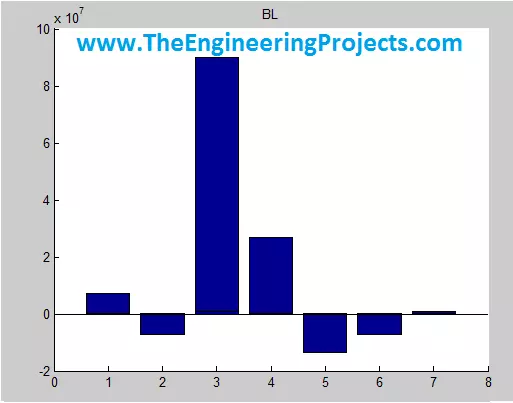
Step 10: Implementation of Black Litterman approach
In this part, I have finally implemented the Black Litterman approach on the data available. Black Litterman approach involves the below steps:
Few MATLAB Projects:
- Send Data to Serial Port in MATLAB
- Speech Recognition using Correlation
- DTMF Decoder using MATLAB
- Hexapod Simulation in MATLAB
- The Covariance Matrix from Historical Data
- Determination of a Baseline Forecast
- Integrating the Manager’s Private Views
- Revised (Posterior) Expectations
- Portfolio Optimization
gamma = 1.9; tau = .3; for w=1:10 ind=[(w-1)*12+1 (w+10)*12]; logRet2=logRet(ind(1):ind(2),:); for i=1:7 OplogRet(:,i)=logRet2(i,:).*xoptCR(i,w)'*100; end covmatOP{1,w}=12*cov(OplogRet); end for w=1:10 Opweig(:,w)=xoptCR(:,w); Pi{w}= gamma *covmatOP{1,w}* Opweig(:,w); end figure for w=1:10 title('BL'); hold on; bar(Pi{w}) hold on; end
