


Types and Operations on Array using NumPy in Python


Hello students! Welcome to the next episode of NumPy, where we are working more on arrays in detail. NumPy is an important library for Python, and for concepts like integer arrays, it has many useful built-in functions that help programmers a lot. In the previous lecture, the installation and basic functions were discussed and this time, our focus is on the general operations and types of arrays that usually the programmers need during the coding. It is an interesting and basic lecture, and you will learn the following concepts in this lecture:
What are some important types of arrays?
Why are we using NumPy for arrays?
What are zero arrays?
What is the random array?
How can we use the ones array using NumPy?
Is it easy to perform the identity array in Numpy?
Practically perform the arithmetic operations in an array.
How do we find the maximum and minimum values in the array?
Important Types of Array with NumPy
If we talk about arrays, it is a vast concept, and many points are important to discuss. It is one of the reasons why we are using the library of numPy and it becomes super easy to work on the arrays using it. There are different types of arrays that we have learned about in our mathematics classes, and some of them are so important that NumPy has special functions for them so that programmers who want to use them do not have to write the whole code manually, but instead, using some important instructions, the array is formed and used automatically according to the instructions.
Zeros Array in Python
Understanding the zeros array is not as difficult as its name implies; it is the array that has all the entries set to zero. In other words, the array does not contain any other value than zero. The size and shape of the array are not restricted by any rules; therefore, any size and shape of the array can be declared as a zero array.
By the same token, the code for some types of arrays is simple and easy, so here we want to show you how some programmers can add random numbers to their arrays by using this simple instruction. So have a look at the syntax, and then we will use it in the code:
For the zero arrays:
myArray =zeros((numbers of rows, numbers of columns))
For adding more details to your array, you can use the following syntax:
myArray = np.zeros( shape , dtype , order )
We are using the zeros array for the first time, therefore, to keep things simple, we will use the first method in our program.
Random Elements of Arrays:
random.rand(numbers of rows, numbers of columns)
Both of these require less effort, but with the help of these built-in functions, the programmers feel the convenience of getting the best result instead of using multiple lines of code to get the required results:
Code:
import numpy as NumPy
#using the zeros method to print the zero array
print("\bZero array with two rows and three columns " )
zeroArray=NumPy.zeros((2,3))
print(zeroArray)
#using the random method to print the array
print("\bThe random array with two rows and three columns ")
randomArray=NumPy.random.rand(2,3)
print(randomArray)
Output:
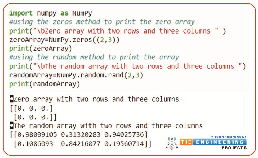
Here, if you have not noticed the syntax, you must see that both of these have similar syntax, but the numbers of brackets are different. If the programmers do not follow the same syntax for each case (for the simple syntax and for the detailed syntax of zero error), then they will face errors.
Now, here is the task for you, check the other syntax mentioned above about the zeros array and try to find out how you can use the other details in your zeros array.
Ones Array using NumPy
The next program to perform is also easy to understand if you know the previous one discussed above. This time, all the entries in the array are one. It means, no other entry other than 1 is the shape of the array can be rectangular, square, or any other according to the requirement of the programmer.
Syntax:
myArray =ones((numbers of rows, numbers of columns))
Code:
#using the ones method to print the ones array
print("\bZero array with two rows and three columns " )
onesArray=NumPy.ones((2,4))
print(onesArray)
# Declaring the array as a tuple
# declaring their data types and printing the results
onesArray = NumPy.ones((2, 3), dtype=[('x', 'int'), ('y', 'float')])
print("\bDetailed ones array= ")
print(onesArray)
print("\bData type of ones array= ")
print(onesArray.dtype)
Output:
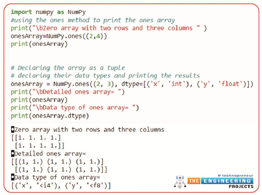
Hence, in this way, we have seen two ways to print our ones array to compare the best method that programmers can use according to their requirements.
Identity Array Using NumPy
The identity array is another important type of matrix or array that is used in multiple instructions, and programmers dealing with numbers must know its formation and applications. We know that the diagonal entries in a matrix or array are the ones that have the same value for row and column. In simple words:
i=j
Where,
i=positions of the row
j=position of the column
So, for the identity array, these rules are followed:
All the diagonal elements are one.
All the elements other than the diagonal are zero.
No other number is used in the diagonal array.
The shape of the diagonal matrix is always square, which means the numbers of rows are equal to the number of columns.
Now it's time to move towards its code and output.
Syntax of Identity Array
myArray=NumPy.identity(integer)
As you can see, only one number is required for this type of array because it is decided that the numbers of rows and columns are equal.
Code for Identity Array
import numpy as NumPy
#declaring an identity array with four rows and four columns.
#printing the simple identity array
print("\bsimple identity matrix")
myArray=NumPy.identity(4)
print(myArray)
#Multiplying the whole array with three.
print("\bAfter the multiplication of the identity matrix with three")
myArray2=3*myArray
print(myArray2)
Output
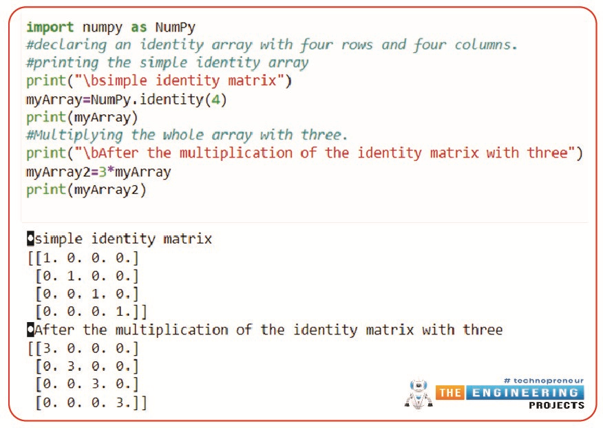
In this way, we have learned that the multiplication of an array is possible in the code, and it is a simple process just as we do it manually in our mathematical problems.
Mathematical Operations on 2D Arrays
When dealing with the arrays, there are certain points that are pros of choosing this data type to manage our data. One of the most prominent advantages is the mathematical operations that can be performed on the arrays by following simple and uncomplicated syntax. Here is the list of the operations that you are going to observe in just a bit on the arrays:
Arithmetic Operations on Arrays
This topic is interesting, and you are going to love it because it is simple to perform and easy to understand but is an important concept in Python, especially when using arrays. We all have been working with addition, subtraction, multiplication, and division since our childhood, and now is the time to use them in arrays. There is no need to explain more, so let’s move towards the code.
Code for Arithmetic Operations on Array
import numpy as NumPy
#Declaring two arrays for the arithmetic operations.
print("\bElements in arrays")
A=NumPy.array([[12,45,11,7],[23,8,11,90],[12,55,1,90]])
print("A= \n", A)
B=NumPy.array([[76,43,1,90],[43,99,14,11],[12,90,22,55]])
print("B= \n", B)
#Performing the arithmetic operations.
print("\bAddition of arrays \n", A+B)
print("\bSubtraction of arrays\n", A-B)
print("\bMultiplication of first array with the second\n", A*B)
print("\bMultiplication of second array with the first\n", B*A)
print("\bDivision of first array with the first\n", A/B)
print("\bDivision of second array with the first\n", B/A)
Output
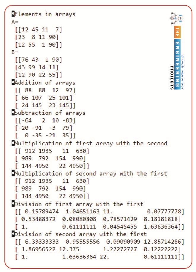
As you can see, we have a long list of outputs, and all the operations that we have discussed are self-explanatory. Here, we have seen that all the arithmetic operations can be done from array to array. Moreover, if you look at both types of multiplication and division, the answers are different, and it makes sense because these arrays do not follow the commutative law when dealing with arrays. Mathematically,
A*B!=B*A
Similarly,
A/B!=B/A
In addition to this, you must know that scaler arithmetic operations can be performed on the array that means, an integer or the float can be added, multiplied, divide and subtracted from the whole matrix, and the effect of that number will be observed on all the entries of that particular array.
Maximum and Minimum of An Array
The next operation in which we are interested in finding the maximum and minimum values in the array. These work great when dealing with image processing and related concepts. These are two different operations, and keep in mind, it seems easy to find the maximum and minimum values in the simple and small arrays, but when talking about the arrays with the order 1000*1000, it becomes almost impossible to find the required value. So without using more time, have a look at the code given next:
The Syntax for Maximum and Minimum Value
maximum_value=numPy.max(Name of the array)
minimu_value=numPy.min(Nmae of the array)
Code for Maximum and Minimum Value
import numpy as NumPy
#Declaring two arrays for the arithmetic operations.
print("\bElements in arrays")
A=NumPy.array([[12,45,11,7],[23,8,11,90],[12,55,1,90]])
print("A= \n", A)
#Finding the maximum Value
maximum=NumPy.max(A)
print("Maximum Value in array = ", maximum)
#Finding the minimum Value
minimum=NumPy.min(A)
print("Minimum Value in array = " ,minimum)
Code:
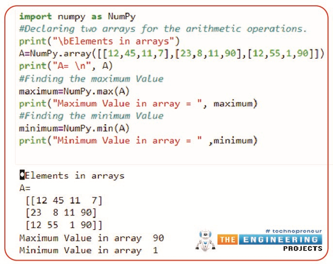
Hence, as you can see, the maximum value occurs more than once in that array, but the compiler only gives us one value. The reason why I am mentioning it is that if NumPy is not used in this case and the programmer does not associate it with the array, the compiler throws the error that there must be another function that has to be used with your particular operation because it takes the array as a tuple. These small details are important to observe because many times, the programmers are stuck into such problems and do not get the reason behind the array.
Syntax of Determinant in NumPy
Determinant=numPy.linalg.det(Name of array)
Code:
import numpy as NumPy
#Declaring two arrays for the arithmetic operations.
print("\bElements in arrays")
A=NumPy.array([[12,45,11,7],[23,8,11,90],[12,55,1,90],[11,33,66,1]])
print("A= \n", A)
#Getting the determinant of the array
determinant =NumPy.linalg.det(A)
print(determinant)
Output:
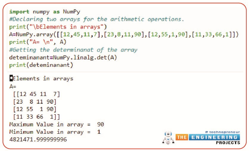
If you are confused with the keyword that we have just used here, let me tell you that linalg is the method in Python that is associated with the determinant of the square array. In other words, as we have used ”random” with the rand function above, there must be the use of linalg with the det function. Moreover, never use these functions with other types of arrays. The determinant can only be used with the square matrix.
Hence, it is enough for today. We have seen a lot of information about the arrays in this lecture, and all of these were performed on the NumPy library. At the start, we saw the types of arrays that the programmers used often in the coding. After that, we saw the mathematical operations such as the arithmetic and general operations in the NumPy. We tried our best to use similar arrays for different operations to make the comparison in our minds. All of these were uncomplicated, and throughout this lecture, we revised the basic concepts of the matrices and arrays that we learned years ago during our early education of computers and mathematics.


